Historical daily weather data from the Global Historical Climate Network (GHCN) is now available in Google BigQuery, our managed analytics data warehouse. The data comes from over 80,000 stations in 180 countries, spans several decades and has been quality-checked to ensure that it’s temporally and spatially consistent. The GHCN daily data is the official weather record in the United States.
According to the National Center for Atmospheric Research (NCAR), routine weather events such as rain and unusually warm and cool days directly affect 3.4% of the US Gross Domestic Product, impacting everyone from ice-cream stores, clothing retailers, delivery services, farmers, resorts and business travelers. The NCAR estimate considers routine weather only — it doesn’t take into account, for example, how weather impacts people’s moods, nor the impact of destructive weather such as tornadoes and hurricanes. If you analyze data to make better business decisions (or if you build machine learning models to provide such guidance automatically), weather should be one of your inputs.
The GHCN data has long been freely available from the National Oceanic and Atmospheric Association (NOAA) website to download and analyze. However, because the dataset changes daily, anyone wishing to analyze that data over time would need to repeat the process the following day. Having the data already loaded and continually refreshed in BigQuery makes it easier for researchers and data scientists to incorporate weather information in analytics and machine learning projects. The fact that BigQuery analysis can be done using standard SQL makes it very convenient to start analyzing the data.
Let’s explore the GHCN dataset and how to interact with it using BigQuery.
Where are the GHCN weather stations?
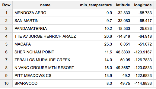
The GHCN data is global. For example, let’s look at all the stations from which we have good minimum-temperature data on August 15, 2016:
SELECT
name,
value/10 AS min_temperature,
latitude,
longitude
FROM
[bigquery-public-data:ghcn_d.ghcnd_stations] AS stn
JOIN
[bigquery-public-data:ghcn_d.ghcnd_2016] AS wx
ON
wx.id = stn.id
WHERE
wx.element = ‘TMIN’
AND wx.qflag IS NULL
AND STRING(wx.date) = ‘2016-08-15′
By plotting the station locations in Google Cloud Datalab, we notice that the density of stations is very good in North America, Europe and Japan and quite reasonable in most of Asia. Most of the gaps correspond to sparsely populated areas such as the Australian outback, Siberia and North Africa. Brazil is the only gaping hole. (For the rest of this post, I’ll show only code snippets — for complete BigQuery queries and Python plotting commands, please see the full Datalab notebook on github.)
Blue dots represent GHCN weather stations around the world.
Using GHCN weather data in your applications
Here’s a simple example of how to incorporate GHCN data into an application. Let’s say you’re a pizza chain based in Chicago and want to explore some weather variables that might affect demand for pizza and pizza delivery times. The first thing to do is to find the GHCN station closest to you. You go to Google Maps and find that your latitude and longitude is 42 degrees latitude and -87.9 degrees longitude, and run a BigQuery query that computes the great-circle distance between a station and (42, -87.9) to get the distance from your pizza shop in kilometers (see the Datalab notebook for what this query looks like). The result looks like this:
Plotting these on a map, you can see that there are a lot of GHCN stations near Chicago, but our pizza shop needs data from station USW00094846 (shown in red) located at O’Hare airport, 3.7 km away from our shop.
Next, we need to pull the data from this station on the dates of interest. Here, I’ll query the table of 2015 data and pull all the days from that table. To get the rainfall amount (“precipitation” or PRCP) in millimeters, you’d write:
SELECT
wx.date,
wx.value/10.0 AS prcp
FROM
[bigquery-public-data:ghcn_d.ghcnd_2015] AS wx
WHERE
id = ‘USW00094846′
AND qflag IS NULL
AND element = ‘PRCP’
ORDER BY wx.date
Note that we divide wx.value by 10 because the GHCN reports rainfall in tenths of millimeters. We ensure that the quality-control flag (qflag) associated with the data is null, indicating that the observation passed spatio-temporal quality-control checks.
Typically, though, you’d want a few more weather variables. Here’s a more complete query that pulls rainfall amount, minimum temperature, maximum temperature and the presence of some weather phenomenon (fog, hail, rain, etc.) on each day:
SELECT
wx.date,
MAX(prcp) AS prcp,
MAX(tmin) AS tmin,
MAX(tmax) AS tmax,
IF(MAX(haswx) = ‘True’, ‘True’, ‘False’) AS haswx
FROM (
SELECT
wx.date,
IF (wx.element = ‘PRCP’, wx.value/10, NULL) AS prcp,
IF (wx.element = ‘TMIN’, wx.value/10, NULL) AS tmin,
IF (wx.element = ‘TMAX’, wx.value/10, NULL) AS tmax,
IF (SUBSTR(wx.element, 0, 2) = ‘WT’, ‘True’, NULL) AS haswx
FROM
[bigquery-public-data:ghcn_d.ghcnd_2015] AS wx
WHERE
id = ‘USW00094846′
AND qflag IS NULL )
GROUP BY
wx.date
ORDER BY
wx.date
The query returns rainfall amounts in millimeters, maximum and minimum temperatures in degrees Celsius and a column that indicates whether there was impactful weather on that day:
You can cast the results into a Pandas DataFrame and easily graph them in Datalab (see notebook in github for queries and plotting code):
BigQuery Views and Data Studio 360 dashboards
Since the previous query pivoted and transformed some fields, you can save the query as a View. Simply copy-paste this query into the BigQuery console and select “Save View”:
SELECT
REPLACE(date,”-“,””) AS date,
MAX(prcp) AS prcp,
MAX(tmin) AS tmin,
MAX(tmax) AS tmax
FROM (
SELECT
STRING(wx.date) AS date,
IF (wx.element = ‘PRCP’, wx.value/10, NULL) AS prcp,
IF (wx.element = ‘TMIN’, wx.value/10, NULL) AS tmin,
IF (wx.element = ‘TMAX’, wx.value/10, NULL) AS tmax
FROM
[bigquery-public-data:ghcn_d.ghcnd_2016] AS wx
WHERE
id = ‘USW00094846′
AND qflag IS NULL
AND value IS NOT NULL
AND DATEDIFF(CURRENT_DATE(), date) < 15 )
GROUP BY
date
ORDER BY
date ASC
Notice my use of DATEDIFF and CURRENT_DATE functions to get weather data from the past two weeks. Saving this query as a View allows me to query and visualize this View as if it were a BigQuery table.
Since visualization is on my mind, I can go over to Data Studio and easily create a dashboard from this View, for example:
One thing to keep in mind is that the “H” in GHCN stands for historical. This data is not real-time, and there’s a time lag. For example, although I did this query on August 25, the latest data shown is from August 22.
Mashing datasets in BigQuery
It’s quite easy to execute a weather query from your analytics program and merge the result with other corporate data.
If that other data is on BigQuery, you can combine it all in a single query! For example, another BigQuery dataset that’s publicly available is airline on-time arrival data. Let’s mash the GHCN and on-time arrivals datasets together:
SELECT
wx.date,
wx.prcp,
f.departure_delay,
f.arrival_airport
FROM (
SELECT
STRING(date) AS date,
value/10 AS prcp
FROM
[bigquery-public-data:ghcn_d.ghcnd_2005]
WHERE
id = ‘USW00094846′
AND qflag IS NULL
AND element = ‘PRCP’) AS wx
JOIN
[bigquery-samples:airline_ontime_data.flights] AS f
ON
f.date = wx.date
WHERE
f.departure_airport = ‘ORD’
LIMIT 100
This yields a table with both flight delay and weather information:
We can look at the distributions in Datalab using the Python package Seaborn:
As expected, the heavier the rain, the more the distribution curves shift to the right, indicating that flight delays increase.
GHCN data in BigQuery democratizes weather data and opens it up to all sorts of data analytics and machine learning applications. We can’t wait to see how you use this data to build what’s next.
Quelle: Google Cloud Platform
Published by