Introducing the Data Validation Tool for EDW migrations

Data validation is a crucial step in data warehouse, database, or data lake migration projects. It involves comparing structured or semi-structured data from the source and target tables and verifying that they match after each migration step (e.g data and schema migration, SQL script translation, ETL migration, etc.) Today, we are excited to announce the Data Validation Tool (DVT), an open sourced Python CLI tool that provides an automated and repeatable solution for validation across different environments. The tool uses the Ibis framework to connect to a large number of data sources including BigQuery, Cloud Spanner, Cloud SQL, Teradata, and more.Why DVT?Cross platform data validation is a non-trivial and time-consuming effort, and many customers have to build and maintain a custom solution to perform such tasks. The DVT provides a standardized solution to validate customer’s newly migrated data in Google Cloud against the existing data from their on-prem systems. DVT can be integrated with existing enterprise infrastructure and ETL pipelines to provide a seamless and automated validation. SolutionThe DVT provides connectivity to BigQuery, Cloud SQL, and Spanner as well as third-party database products and file systems. In addition, it can be easily integrated into other Google Cloud services such as Cloud Composer, Cloud Functions and Cloud Run. DVT supports the following connection types:BigQueryCloud SQLFileSystem (GCS, S3, or local files)HiveImpalaMySQLOraclePostgresRedshiftSnowflakeSpannerSQL ServerTeradataThe DVT performs multi-leveled data validation functions, from the table level all the way to the row level. Below is a list of the validation features:Table levelTable row countGroup by row countColumn aggregationFilters and limitsColumn levelSchema/Column data type Row level Hash comparison (BigQuery only)Raw SQL explorationRun custom queries on different data sourcesHow to Use the DVTThe first step to validating your data is creating a connection. You can create a connection to any of the data sources listed previously. Here’s an example of connecting to BigQuery:Now you can run a validation. This is how a validation between a BigQuery and a MySQL table would look:The default validation if no aggregation is provided is a COUNT *. The tool will count the number of columns in the source table and verify it matches the count on the target table.The DVT supports a lot of customization while validating your data. For example, you can validate multiple tables, run validations on specific columns, and add labels to your validations.You can also save your validation to a YAML configuration file. This way you can store previous validations and modify your validation configuration. By providing the `config-file` flag, you can generate the YAML file. Note that the validation will not execute when this flag is provided – only the file is created.Here is an example of a YAML configuration file for a GroupedColumn validation:Once you have a YAML configuration file, it is very easy to run the validation.Validation reports can be output to stdout (default) or to a result handler. The tool currently supports BigQuery as the result handler. In order to output to BigQuery, simply add the `–bq-result-handler` or `-bqrh` flag.Below is an example of the validation results in BigQuery. View the complete schema for validation reports in BigQuery here.Getting StartedReady to start integrating the DVT into your data movement processes? Check out the tool on PyPi here and contribute to the tool via GitHub. We’re actively working on new features to make the tool as useful to our customers. Happy validating!Related ArticleHighway to the landing zone: Google Cloud migration made easyMigration to cloud is the first step to digital transformation because it offers a quick, simple path to cost savings and enhanced flexib…Read Article
Quelle: Google Cloud Platform

Staying ahead with API-powered Application Innovation

Modern tech-savvy customers today are looking for digital-first, connected, and seamless business interactions. And businesses are looking not only to keep up with the fast-changing customer expectations but also maintain their profitability. They must find ways to balance both by leaning into sustainable innovation across every aspect of business. Innovation at speed is easier said than done, especially when you have legacy systems to manage, when you face a shortage of skilled resources, or when your business is operating in silos. This is where application programming interfaces, or APIs come into the picture, as application innovation is achievable at a significantly faster rate when it’s fueled by APIs. They are like the foundational building blocks that make it easy to deliver modern digital experiences, connect siloed units and systems, and help realize the true business value of your investments.How APIs can take on large-scale app innovationYou may know APIs as small lines of code, but they play a large role in powering app innovation in today’s digital age. Those small lines of code let developers access data and functionality in different systems, which turns those digital assets into modular building blocks that let your enterprise try new things and link together different parts of the buyer’s journey. APIs are inherently made to connect – and be connected – whether the link is between different parts of your business, from your business to a myriad of devices from tablets to computers to smart watches, third-party partners, marketplaces, data analysis tools, or from your business to developer communities. When designed and managed for reuse and developer consumption, APIs help businesses  innovate at scale by combining digital assets to create engaging, unique, and personalized experiences for customers, for example: opting for contactless curbside pickup, collecting and redeeming loyalty points across channels, or getting product recommendations based on shopping behaviors  . Plus, APIs come with an added bonus. Businesses can choose to package their valuable assets as APIs so that they can be monetized, and sold just like any product you’d find on a store shelf—which means if you have a particularly popular and valuable data or service, outsiders may be interested in purchasing access. To build and scale your API program, an API management platform, like Google Cloud’s Apigee, is key. APIs are the access points for many of your business’s most valuable systems, so access needs to be managed, usage needs to be understood, performance needs to be maintained, and security must be continually bolstered. Apigee manages your APIs all in one place, allowing you to design, iterate, deploy, secure, analyze, and scale your APIs from cradle to grave. The innovation we are describing isn’t an abstract concept, just like the notion of the technology “cloud” isn’t an imaginary untappable place in the sky that stores pictures of you from ten years ago. To help demystify, we’ve broken down API-powered application innovation into a three-phase journey:Deliver personalized experiences consistently at scaleAPIs enable companies – regardless of size – to build and deliver personalized experiences for customers. An API-first architecture simplifies how developers can build customizable experiences and thereby reduces time to market for new products and services. Imagine your team has built an API for your call center which recommends new products based on the customer’s profile. That API isn’t limited to that one, initial purpose but can also be embedded into other places and technologies such as your mobile device, app, and/or voice app. When built more efficiently and faster with APIs, these experiences can become more personalized, adaptable, and consistent.Build powerful digital business ecosystems By securely sharing your APIs with partners outside your business, you can unlock a range of ecosystem strategies that stretch and scale the value of your innovations. By making your APIs available to third parties, you can increase the number of innovators harnessing your digital assets, potentially exposing your business to new customers and use cases that wouldn’t have developed through internal innovation alone. Likewise, by combining your data and functionality with third-party APIs, your business and its partners can symbiotically produce more value together than either can by itself. For instance, partners can securely leverage your company’s proprietary data, accessible as an API, along with their expertise to create unique experiences for customers that you may not be able to reach on your own. APIs can be connected to, securely shared with, and even packaged and sold to developers, partners, and customers, allowing you to both deepen the integration with other companies and grow your revenue streams. As the owner of your APIs, you’re able to retain control of what is shared with whom, letting you maintain security while still leaving appropriate partners free to innovate with your data.  Power your innovation with dataAs great digital experiences roll out to customers and APIs gain traction throughout your business ecosystems, you can use API management capabilities to measure and analyze API usage data, letting you optimize innovations and iterate on the cycle again and again. APIs make it simple and secure to share desired data insights with suppliers, customers, and partners to foster more innovation. In other words, APIs not only link data to data and data to people, but also provide you and your business with established data aggregation and analysis tools. Data-powered innovation enables you to make more informed data-driven decisions for your business and derive maximum value from your APIs and the connections they forge. What’s Stopping You? Start Here.To ensure every business is equipped with the knowledge and tools needed to innovate, Google Cloud is releasing a series that expands upon the three pillars of API-powered Application Innovation. If you’re ready to embark on a journey of innovation, watchthe first Application Innovation webinar in our series.Related ArticleRead Article
Quelle: Google Cloud Platform

Query BIG with BigQuery: A cheat sheet

Organizations rely on data warehouses to aggregate data from disparate sources, process it, and make it available for data analysis in support of strategic decision-making. BigQuery is the Google Cloud enterprise data warehouse designed to help organizations to run large scale analytics with ease and quickly unlock actionable insights. You can ingest data into BigQuery either through batch uploading or by streaming data directly to unlock real-time insights. As a fully-managed data warehouse, BigQuery takes care of the infrastructure so you can focus on analyzing your data up to petabyte-scale. BigQuery supports SQL (Structured Query Language), which you’re likely already familiar with if you’ve worked with ANSI-compliant relational databases. Click to enlargeBigQuery unique featuresBI Engine – BigQuery BI Engine is a fast, in-memory analysis service that provides subsecond query response times with high concurrency. BI Engine integrates with Google Data Studioand Looker for visualizing query results and enables integration with other popular business intelligence (BI) tools. BigQuery ML: BigQuery ML is unlocking machine learning for millions of data analysts. It  enables data analysts and data scientists to build and operationalize machine learning models directly within BigQuery, using simple SQL.Click to enlargeBigQuery Omni – BigQuery Omni is a flexible, multi-cloud analytics solution powered by Anthos that lets you cost-effectively access and securely analyze data across Google Cloud, Amazon Web Services (AWS), and Azure, without leaving the BigQuery user interface (UI). Using standard SQL and familiar BigQuery APIs, you can break down data silos and gain critical business insights from a single pane of glass. Data QnA: Data QnA enables self-service analytics for business users on BigQuery data as well as federated data from Cloud Storage, Bigtable, Cloud SQL, or Google Drive. It uses Dialogflow and enables users to formulate free-form text analytical questions, with auto-suggested entities while users type a question.Connected Sheets -The native integration between Sheets and BigQuery makes it possible for all business stakeholders, who are already quite familiar with spreadsheet tools, to get their own up-to-date insights at any time.Geospatial data – BigQuery offers accurate and scalable geospatial analysis with geography data types. It supports core GIS functions – measurements, transforms, constructors, and more – using standard SQL.How does it work?Here’s how it works: You ingest your own data into BigQuery or use data from the public datasets. Storage and compute are decoupled and can scale independently on demand. This offers immense flexibility and cost control for your business as you don’t need to keep expensive compute resources up and running all the time. As a result, BigQuery is much more cost-effective than traditional node-based cloud data warehouse solutions or on-premises systems. BigQuery also provides automatic backup and restore of your data. You can ingest data into BigQuery in batches or stream real-time data from web, IoT, or mobile devices via Pub/Sub. You can also use Data Transfer Service to ingest data from other clouds, on-premises systems or third-party services. BigQuery also supports ODBC and JDBC drivers to connect with existing tools and infrastructure. Interacting with BigQuery to load data, run queries, or create ML models can be done in three different ways. You can use the UI in the Cloud Console, the BigQuery command-line tool, or the API via client libraries available in several languages.When it comes time to visualize your data, BigQuery integrates with Looker as well as several other business intelligence tools across the Google partner ecosystem.What about security?BigQuery offers built-in data protection at scale. It provides security and governance tools to efficiently govern data and democratize insights within your organization. Within BigQuery, users can assign dataset-level and project-level permissions to help govern data access. Secure data sharing ensures you can collaborate and operate your business with trust.Data is automatically encrypted both while in transit and at rest, ensuring that your data is protected from intrusions, theft, and attacks. Cloud DLP helps you discover and classify sensitive data assets.Cloud IAM provides access control and visibility into security policies.Data Catalog helps you discover and manage data. How much does it cost?The BigQuery sandbox lets you explore BigQuery capabilities at no cost and confirm that BigQuery fits your needs. With BigQuery you get predictable price-performance: you pay for storing and querying data, and for streaming inserts. Loading and exporting data are free of charge. Storage costs are based on the amount of data stored, and have two rates based on how often the data is changing. Query costs can be either:On-demand – you are charged per query by the amount of data processedFlat-rate – if you prefer to purchase dedicated resources You can start with the pay-as-you-go, on-demand option and later move to flat-rate if that better suits your usage. Or, start with flat-rate, get a better understanding of your usage and move to the pay-as-you-go models for additional workloads. To explore BigQuery and its capabilities a bit more, check out the sandbox; and when you’re ready to modernize your data warehouse with BigQuery then check out the documentation to streamline your migration process here. For more #GCPSketchnote, follow the GitHub repo. For similar cloud content follow me on Twitter @pvergadia and keep an eye out on thecloudgirl.dev.Related ArticleBigtable vs. BigQuery: What’s the difference?Bigtable vs BigQuery? What’s the difference? In this blog, you’ll get a side-by-side view of Google BigQuery and Google Cloud Bigtable.Read Article
Quelle: Google Cloud Platform

Make informed decisions with Google Trends data

A few weeks ago, we launched a new dataset into Google Cloud’s public dataset program: Google Trends. If you’re not familiar with our datasets program, we host a variety of datasets in BigQuery and Cloud Storage for you to access and integrate into your analytics. Google pays for the storage of these datasets and provides public access to the data, e.g., via the bigquery-public-data project. You only pay for queries against the data. Plus, the first 1 TB per month is free! Even better, all of these public datasets will soon be accessible and shareable via Analytics Hub. The Google Trends dataset represents the first time we’re adding Google-owned Search data into the program. The Trends data allows users to measure interest in a particular topic or search term across Google Search, from around the United States, down to the city-level. You can learn more about the dataset here, andcheck out the Looker dashboard here! These tables are super valuable in their own right, but when you blend them with other actionable data you can unlock whole new areas of opportunity for your team. You can view and run the queries we demonstrate here.Focusing on areas that matterEach day, the top 25 search terms are added to the top_terms table. Additionally, information about how that term has fluctuated over time for each region, Nielsen’s Designated Market Area® (DMA), is recorded with a score. A value of 100 is the peak popularity for the term. This regional information can offer further insight into trends for your organization.Let’s say I have a BigQuery table that contains information about each one of my physical retail locations. Like we mentioned in our previous blog post, depending on how that data is brought into BigQuery we might enhance the base table by using the Google Maps Geocoding API to convert text-based addresses into lat-lon coordinates.So now how do I join this data with the Google Trends data? This is where BigQuery GIS functions, plus the public boundaries dataset comes into play. Here I can use the DMA table to determine which DMA each store is in. From there I can simply join back onto the trends data using the DMA ID and focus on the top three terms for each store, which is based on terms with the highest score for that area within the past week.With this information, you can figure out what trends are most important to customers in the areas you care about, which can help you optimize marketing efforts, stock levels, and employee coverage. You may even want to compare across your stores to see how similar term interest is, which may offer new insight into localized product development. Filtering for relevant search termsSearch terms are constantly changing and it might not be practical for your team to dig into each and every one.  Instead, you might want to focus your analysis on terms that are relevant to you. Let’s imagine that you have a table that contains all your product names. These names can be long and may contain lots of words or phrases that aren’t necessary for this analysis. For example:“10oz Authentic Ham and Sausages from Spain”Like most text problems, you should probably start with some preprocessing. Here, we’re using a simple user-defined functionthat converts the string to lowercase, tokenizes it, and removes words with numbers, and stop words or adjectives that we’ve hard-coded.For a more robust solution, you might want to leverage a natural language processing package, for example NLTK in Python. You can even process words to use only the stem or find some synonyms to include in your search. Next, you can join the products table onto the trends data, selecting search terms that contain one of the words from the product name.It looks like `Spain vs Croatia` was recently trending because of the Euro Cup. This might be a great opportunity to create a new campaign and capitalize on momentum: “Spain beat Croatia and is on to the next round, show your support by celebrating with some authentic Spanish ham!” Now going a bit further, if we take a look at the top rising search terms from yesterday (as of writing this on 6/30), we can see that there are a lot of names for people.  But it’s unclear who  these people are or why they’re trending. What we do know is we’re looking for a singer to strike up a brand deal with. More specifically, we have a great new jingle for our authentic ham and we’re looking for some trendy singers to bring attention to our company.Using the Wikipedia Open API you can perform an open search for the term, for example “Jamie Lynn Spears”:https://en.wikipedia.org/w/api.php?action=opensearch&search=jamie+lynn+spears&limit=1&namespace=0&format=json This gives you a JSON response that contains the name of first wikipedia page returned in the search, which you can then use to perform a query against the API:https://en.wikipedia.org/w/api.php?action=query&prop=extracts&exintro&titles=Jamie_Lynn_Spears&format=jsonFrom here you can grab the first sentence on the page (hint: this usually tells us if the person in question is a singer or not):  “Jamie Lynn Marie Spears (born April 4, 1991) is an American actress and singer.”Putting this together, we might create a Google Cloud functionthat selects new BigQuery search terms from the table, calls the wikipedia API for each of them, grabs that first sentence and searches for the word “singer.” If we have a hit, then we simply add the search term to the table.Check out some sample code here! Not only does this help us keep track of who the most trendy singers are, but we can use the historical scores to see how their influence has changed over time. Staying notifiedThese queries, plus many more, can be used to make various business decisions. Aside from looking at product names, you might want to keep tabs on competitor names so that you can begin a competitive analysis against rising challengers in your industry. Or maybe you’re interested in a brand deal with a sports player instead of a singer, so you want to make sure you’re aware of any rising stars in the athletic world.  Either way you probably want to be notified when new trends might influence your decision making. With another Google Cloud Function, you can programmatically run any interesting SQL queries and return the results in an email. With Cloud Scheduler, you can make sure the function runs each morning, so you stay alert as new trends data is added to the public dataset. Check out the details on how to implement this solution here. Ready to get started?You can explore the new Google Trends dataset in your own project, or if you’re new to BigQuery spin up a project using the BigQuery sandbox. The trends data, along with all the other Google Cloud Public Datasets, will be available in Analytics Hub – so make sure to sign up for the preview, which is scheduled to be available in the third quarter of 2021, by going to g.co/cloud/analytics-hub.Related ArticleMost popular public datasets to enrich your BigQuery analysesCheck out free public datasets from Google Cloud, available to help you get started easily with big data analytics in BigQuery and Cloud …Read Article
Quelle: Google Cloud Platform

How to put your company on a path to successful cloud migration

Migrating your company’s applications to the cloud has many benefits, including improved customer satisfaction, reduction of technical debt, and the ability to lay the foundations of operational excellence. But there are also many challenges. Organizations often stop short because they don’t know how to get started, lacking prescriptive guidance and partnership from their cloud provider. In our new white paper, we hope to provide simple, direct guidance to help with the most important part of your digital transformation: the beginning. Application migration can be challenging because there isn’t a one-size-fits-all solution – every digital transformation has its own nuances and unique considerations. Before starting out on this journey, you need to understand the advantages and disadvantages of the options available to you, so you can create a migration plan that makes the most sense for your business. That’s why we’ve outlined the benefits of different migration paths to help you decide what’s right for your organization, the options of which you can see in the diagram below: Cloud migration options diagramAt Google Cloud, we’re here to help make sure your migration goes successful from start to finish (and beyond)! To learn more, download this white paper. Or, if you’re really ready to jump start your migration today, you can take advantage of our current offer by signing up for a free discovery and assessment or exploring our Rapid Assessment and Migration Program (also known as RAMP).
Quelle: Google Cloud Platform

Kickstart your organization’s ML application development flywheel with the Vertex Feature Store

We often hear from our customers that over 70% of the time spent by Data Scientists goes into wrangling data. More specifically, the time is spent in feature engineering — the transformation of raw data into high quality input signals for machine learning (ML) models — and in reliably deploying these ML features in production. However, today, this process is often inefficient and brittle.There are three key challenges with regards to ML features that come up often: Hard to share and reuseHard to serve in production, reliably with low latencyInadvertent skew in feature values between training and serving In this blog post, we explain how the recently launched Vertex Feature Store helps address the above challenges. It helps enterprises reduce the time to build and deploy AI/ML applications by making it easy to manage and organize ML features. It is a fully managed and unified solution to share, discover, and serve ML features at scale, across different teams within an organization.Vertex Feature Store solves the feature management problemsSimple and easy to useAs illustrated in the overview diagram below, Vertex Feature Store uses a combination of storage systems and components under the hood. However, our goal is to abstract away the underlying complexity and deliver a managed solution that exposes a few simple APIs and corresponding SDKs. High level animated illustration of the Feature StoreThe key APIs are:Batch Import API to ingest computed feature values. We will soon be launching a Streaming Import API as well. When a user ingests feature values via an ingestion API, the data is reliably written both to an offline store and to an online store. The offline store will retain feature values for a long duration of time, so that they can later be retrieved for training. The online store will contain the latest feature values for online predictions.Online Serving API to serve the latest feature values from the online store, with low latency. This API will be used by client applications to fetch feature values to perform online predictions.Batch Serving API to fetch data from the offline store, for training a model or for performing batch predictions. To fetch the appropriate feature values for training, the Batch Serving API performs “point-in-time lookups”, which are described in more detail below.Now lets do a deeper dive into how the Feature Store addresses the three challenges mentioned above.Making it easy to discover, share, and re-use featuresReducing redundancy: Within a broader organization, it is common for different machine learning use cases to have some identical features as inputs to their models. In the absence of a feature store, each team invariably does the work of authoring and maintaining their own feature engineering pipelines, even for the identical features. This is redundant work, reducing productivity, that can be avoided.Maximizing the impact of feature engineering efforts: Coming up with sophisticated high quality features entails non-trivial creativity and effort. A high quality feature can often add value across many diverse use cases. However, when the feature goes underutilized, it is a lost opportunity for the organization. Hence, it is important to make it easy for different teams to share and re-use their ML features.Vertex Feature Store can serve as a shared feature repository for the entire organization. It provides an intuitive UI and APIs to search and discover existing features. Access to the features can also be controlled by setting appropriate permissions over groups of features.Discovery without trust is not very useful. Hence, Vertex Feature Store provides metrics that convey information about the quality of the features, such as: What is the distribution of the feature values? How often are a particular feature’s values updated? How widely is the feature consumed by other teams?Feature monitoring on the Feature Store consoleMaking it easy to serve ML features in productionMany compelling machine learning use cases deploy their models for online serving, so that predictions can be served in real-time with low latency. The Vertex Prediction service makes it easy to deploy a model as an HTTP or RPC endpoint, at scale, with high availability and reliability. However, in addition to deploying the model, the features required by the model as inputs need to be served online. Today, in most organizations there is a disconnect: it is the Data Scientist that creates new ML features, but the serving of ML features is handled by Ops or Engineering teams. This makes Data Scientists dependent on other teams to deploy their features in production. This dependence causes an undesirable bottleneck. Data Scientists would prefer to be in control of the full ML feature lifecycle. They want the freedom and agility to create and deploy new features quickly.  Vertex Feature Store gives Data Scientists autonomy by providing a fully-managed and easy to use solution for scalable, low-latency online feature serving. Simply use the Ingestion APIs to ingest new feature values to a feature store. Once ingested, they are ready for online serving. Mitigating training-serving skewIn real world machine learning applications, one can run into a situation where a model performs very well on offline test data, but fails to perform as expected when deployed in production. This is often called Training-Serving Skew. While there can be many nuanced causes of model training-serving skew, often it boils down to skew between the features provided to the model during training and the features provided while making predictions.At Google, there is a rule of thumb to avoid training-serving skew: you train like you serve.A rule for mitigating training-serving skew(from Rules of Machine Learning)Discrepancies between the features provided to the model during training and serving are predominantly caused by the following three issues:A. Different code paths for generating features for training and serving. If there are different code paths, inadvertently some deviations can creep inB. A change in the raw data between when the model was trained and when it is subsequently used in production. This is called data drift and often impacts long-running models.C. A feedback loop between your model and your algorithm, also called data leakage or target leakage. Please read the following two links for a good description of this phenomenon:     a. https://www.kaggle.com/dansbecker/data-leakage     b. https://cloud.google.com/automl-tables/docs/beginners-guide#prevent_data_leakage_and_training-serving_skewLet’s see how Vertex Feature Store addresses the aforementioned three causes of feature skew:The feature store addresses (A) by ensuring that a feature value is ingested once into Vertex Feature Store, and then re-used for both training and serving. Since the feature value is only computed once, it avoids discrepancy due to duplicate code paths. (B) is addressed by constantly monitoring the distributions of feature values ingested into the feature store, so that users can identify when the feature values start to drift and change over time.(C) is addressed by what we call “point-in-time lookups” of features for training. This is described in more detail below. Essentially, this addresses data-leakage by ensuring that feature values provided for training were computed prior to the timestamp of the corresponding labeled training instance. The labelled instances used for training a model correspond to events that occurred at a specific time. As described by the data leakage links above, information generated after the label event should not be incorporated into the corresponding features. After all, that would effectively constitute “peeking” into the future:Point-in-time lookups to fetch training dataFor model training, you need a training data set that contains examples of your prediction task. These examples consist of instances that include their features and labels. For example, an instance might be a home and you want to determine its market value. Its features might include its location, age, and the prices of nearby homes that were sold. A label is an answer for the prediction task, such as the home eventually sold for $100K.Because each label is an observation at a specific point in time, you need to fetch feature values that correspond to that point in time when the observation was made, like what were the prices of nearby homes when a particular home was sold. As labels and feature values are collected over time, those feature values change. Hence, when you fetch data from a feature store for model training, it performs point-in-time lookups to fetch the feature values corresponding to the time of each label. What is noteworthy is that the Feature Store performs these point-in-time lookups efficiently, even when the training dataset has tens of millions of labels.In the following example, we want to retrieve feature values for two training instances with labels L1 and L2. The two labels are observed at time T1 and T2, respectively. Imagine freezing the state of the feature values at those timestamps. Hence, for the point-in-time lookup at T1, Vertex Feature Store returns the latest feature values up to time T1 for Feature 1, Feature 2, and Feature 3 and does not leak any values past T1. As time progresses, the feature values change and, consequently, so does the label. So, at T2, Vertex Feature Store returns different feature values for that point in time.Point-in-time Lookup for preventing the data leakA virtuous flywheel for faster AI/ML application developmentA rich feature repository can kick start a virtuous flywheel effect that can significantly reduce the time and cost of building and deploying ML applications. With Vertex Feature Store, Data Scientists don’t need to start from scratch, rather they can build each ML application faster by discovering and reusing features created for prior applications. Moreover, Vertex Feature Store ensures maximum return on investment for each newly crafted feature, ensuring that it benefits the entire organization and further speeds up subsequent applications, leading to a virtuous flywheel effect.Kick start your AI/ML flywheel by following the tutorials and getting started samples in the product documentation.Related ArticleGoogle Cloud unveils Vertex AI, one platform, every ML tool you needGoogle Cloud launches Vertex AI, a managed platform for experimentation, versioning and deploying ML models into production.Read Article
Quelle: Google Cloud Platform

Inside Chess.com's smart move to Google Cloud

Editors note: In early 2020, Chess.com was experiencing steady growth and had projected that it would hit around 4 million daily active users in 10 years. Then the pandemic hit, and alongside the release of the Netflix smash hit, The Queen’s Gambit, they reached this active user number in six months. In this post, Saad Abdali, Director of Technology at Chess.com, explains how handling this surge would have been impossible without the help of their migration to Google Cloud. Happy International Chess Day! Chess is often seen as a game that’s elitist and stodgy —something your grandfather played back in the day. In fact, nothing could be further from the truth. Thanks to the internet and sites like ours, chess has never been more vibrant than it is today.Each day, millions of people visit Chess.com to learn the game, solve puzzles, play against similarly skilled opponents, watch live tournaments, and connect with other chess aficionados. During the pandemic, interest in the sport grew faster than at any time in history.  By adopting Google Cloud, we have been able to achieve things that were difficult or impossible when relying solely on our on-premise hardware. The greatest benefit Google Cloud provides is the ability to scale instantly as demand increases. And in 2020, the demand for online chess surged in a way we had never seen before.Controlling the boardWe first began noticing unpredictable spikes in traffic when our weekly Titled Tuesday event began surging in popularity in 2019. Titled Tuesday is a contest where the best players in the world (those who have the title of Master or better) compete in high-stakes one-hour matches for prize money. We introduced the event in 2014, and by 2018 the event was attracting nearly 400 of the chess world’s brightest stars each week, along with the legions of fans who wanted to watch them play.. Keeping our on-premise servers up and running during these increasingly high-stakes events was a growing challenge.Then the pandemic hit. Almost overnight, traffic to Chess.com tripled. Since our launch in 2007, we had been growing at a steady rate of about 20-50% every year. But in March 2020 alone, our number of daily active users rose from 280,000 to more than 1 million. Fortunately for us, we’d begun migrating significant functionality to Google Cloud in mid-2019. Before then, we’d run entirely on hardware we owned and deployed to physical data centers. So when our traffic surged, we were able to click a few buttons and spin up all the virtual servers we needed. A new gambit Traffic remained at that high level throughout the summer and early fall. And then, after The Queen’s Gambit debuted on Netflix last November, it doubled again. The fictional story of Beth Harmon’s rise to chess mastery inspired a new generation of players, especially young women. At the peak, we were serving up to 6 million users each day. The surge in popularity inspired us to create chess-playing bots that use a Monte Carlo tree search system to mimic Harmon’s style of play, as well as the styles of living grandmasters like Hikaru Nakamura and Maxime Vachier-Lagrave.Our ability to quickly expand capacity with Google Cloud is what allowed Chess.com to meet all of that rapidly increasing demand. It also enabled us to roll out new game types, like Puzzle Battle, where players compete against similarly skilled opponents to solve a series of increasingly complex chess problems. Puzzle Battle was the first major feature that we designed from the ground up to run in Google Cloud. Not only did this avoid adding load to our on-premise hardware, but we found that it significantly accelerated the development process. We’re currently migrating all gameplay from Chess.com, as well as its companion site, ChessKid.com, to a new distributed gameplay system hosted entirely on Google Cloud. In addition to helping us scale, the new cloud architecture provides a number of other benefits, including the ability to deploy a truly global service. One of the most popular game types on Chess.com is Bullet Chess, in which each player gets just one minute on the clock; these extremely fast games are quite time-sensitive. Google Cloud is enabling us to deploy gameplay nodes across the world, so that each player can enjoy a low-latency connection to a nearby Chess.com node.Check and mate After The Queen’s Gambit, our site traffic stabilized to around 4 million daily active users. Still, the site experienced 10 years’ worth of projected growth in just six months. There is no way Chess.com could have handled that surge without the move to Google Cloud. With Google Cloud’s nearly infinite ability to scale in response to demand, we don’t have to forecast what our site traffic is going to be at any point in time. We no longer worry about whether the site is resilient enough to withstand unexpected surges, or end up wasting money by over-provisioning servers that go unused. It also gives us the freedom to experiment with new projects at minimal risk. We can try out new features for the site. If they fail, we can spin down the virtual machines and stop paying for them. If they are a wild success, we can simply add more machines to spread the load. Our greater mission is to share our love of chess with the world, and to enable existing players to expand their horizons. It’s one of the reasons why we’ve created sites like ChessKid.com, and recently together with The International Chess Federation (FIDE), announced the first-ever Women’s World Cup.Chess began as a game, turned into a community, and is becoming a movement. We’re proud of the role Chess.com has played in that evolution, and grateful for the help Google Cloud has provided in allowing us to make it a reality.Related ArticleBringing Pokémon GO to life on Google CloudThroughout my career as an engineer, I’ve had a hand in numerous product launches that grew to millions of users. User adoption typically…Read Article
Quelle: Google Cloud Platform

Scaling deep learning workloads with PyTorch / XLA and Cloud TPU VM

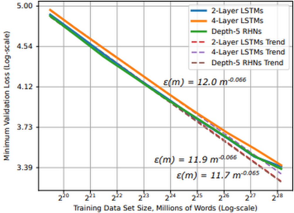
IntroductionMany deep learning advancements can be attributed to increases in (1) data size and (2) computational power. Training deep learning models with larger datasets can be extremely beneficial for model training. Not only do they help stabilize model performance during training, but research shows that for moderate to large-scale models and datasets, model performance converges as a power-law with training data size, meaning we can predict improvements to model accuracy as the dataset grows.Figure 1: Learning curve and dataset size for word language models (source)In practice this means as we look to improve model performance with larger datasets, (1) we need access to hardware accelerators, such as GPUs or TPUs, and (2) we need to architect a system that efficiently stores and delivers this data to the accelerators. There are a few reasons why we may choose to stream data from remote storage to our accelerator devices:Data size: data can be too large to fit on a single machine, requiring remote storage and efficient network accessStreamlined workflows: transferring data to disk can be time consuming and resource intensive, we want to make fewer copies of the data Collaboration: disaggregating data from accelerator devices means we can more efficiently share accelerator nodes across workloads and teamsStreaming training data from remote storage to accelerators can alleviate these issues, but it introduces a host of new challenges:Network overhead: Many datasets consist of millions of individual files, randomly accessing these files can introduce network bottlenecks. We need sequential access patternsThroughput: Modern accelerators are fast; the challenge is feeding them fast enough to keep them fully utilized. We need parallel I/O and pipelined access to dataRandomness vs Sequential: The optimization algorithms in deep learning jobs benefit from randomness, but random file access introduces network bottlenecks. Sequential access alleviates network bottlenecks, but can reduce the randomness needed for training optimization. We need to balance these How do we architect a system that addresses these challenges at scale?Figure 2: Scaling to larger datasets, more devices In this post, we will cover:The challenges associated with scaling deep learning jobs to distributed training settingsUsing the new Cloud TPU VM interfaceHow to stream training data from Google Cloud Storage (GCS) to PyTorch / XLA models running on Cloud TPU Pod slicesYou can find accompanying code for this article in this GitHub repository. Model and datasetIn this article, we will train a PyTorch / XLA ResNet-50 model on a v3-32 TPU Pod slice where training data is stored in GCS and streamed to the TPU VMs at training time. ResNet-50 is a 50-layer convolutional neural network commonly used for computer vision tasks and machine learning performance benchmarking. To demonstrate an end-to-end example, we will use the CIFAR-10 dataset. The original dataset consists of 60,000 32×32 color images divided into 10 classes, each class containing 6,000 images. We have upsampled this dataset, creating a training and test set of 1,280,000 and 50,000 images, respectively. CIFAR is used because it is publicly accessible and well known; however, in the GitHub repository, we provide guidance for adapting this solution to your workloads, as well as larger datasets such as ImageNet.Cloud TPUTPUs, or Tensor Processing Units, are ML ASICs specifically designed for large-scale model training. As they excel at any task where large matrix multiplications dominate, they can accelerate deep learning jobs and reduce the total cost of training. If you’re new to TPUs, check this article to understand how they work. The v3-32 TPU used in this example consists of 32 TPU v3 cores and 256 GiB of total TPU memory. This TPU Pod slice consists of 4 TPU Boards (a Board has 8 TPU cores). Each TPU Board is connected to a high-performance CPU-based host machine for things like loading and preprocessing data to feed to the TPUs.Figure 3: Cloud TPU VM architecture (source)We will access the TPU through the new Cloud TPU VMs. When we use Cloud TPU VMs, a VM is created for each TPU board in the configuration. Each VM consists of 48 vCPUs and 340 GB of memory, and comes preinstalled with the latest PyTorch / XLA image. Because there is no user VM, we ssh directly into the TPU host to run our model and code. This root access eliminates the need for a network, VPC, or firewall between our code and the TPU VM, which can significantly improve the performance of our input pipeline. For more details on Cloud TPU VMs, see the System Architecture.PyTorch / XLAPyTorch / XLA is a Python library that uses the XLA (Accelerated Linear Algebra) deep learning compiler to connect PyTorch and Cloud TPUs. Check out the GitHub repository for tutorials, best practices, Docker Images, and code for popular models (e.g., ResNet-50 and AlexNet).Data parallel distributed trainingDistributed training typically refers to training workloads which use multiple accelerator devices (e.g. GPU or TPU). In our example, we are executing a data parallel distributed training job with stochastic gradient descent. In data parallel training, our model fits on a single TPU device and we replicate the model across each device in our distributed configuration. When we add more devices, our goal is to reduce overall training time by distributing non-overlapping partitions of the training batch to each device for parallel processing. Because our model is replicated across devices, the models on each device need to communicate to synchronize their weights after each training step. In distributed data parallel jobs, this device communication is typically done either asynchronously or synchronously.Cloud TPUs execute synchronous device communication over the dedicated high-speed network connecting the chips. In our model code, we use PyTorch / XLA’s optimizer_step(optimizer) to calculate the gradients and initiate this synchronous update.Figure 4: Synchronous all-reduce on Cloud TPU interconnectAfter the local gradients are computed, the xm.optimizer_step() function synchronizes the local gradients between cores by applying an AllReduce(SUM) operation, and then calls the PyTorch optimizer_step(optimizer), which updates the local weights with the synchronized gradients. On the TPU, the XLA compiler generates AllReduce operations over the dedicated network connecting the chips. Ultimately, the globally averaged gradients are written to each model replica’s parameter weights, ensuring the replicas start from the same state in every training iteration. We can see the call to this function in the training loop: Input pipeline performanceAs previously mentioned, the challenge with TPUs is feeding them the training data fast enough to keep them busy. This problem exists when we store training data on a local disk and becomes even more clear when we stream data from remote storage. Let’s first review a typical machine learning training loop.Figure 5: Common machine learning training loop and hardware configurationIn this illustration, we see the following steps:Training data is either stored on local disk or remote storage The CPU (1) requests and reads the data, augments it with various transformations, batches it, and feeds it to the model Once the model has the transformed, batched training data, (2) the accelerator takes over The accelerator (2a) computes the forward pass, (2b) loss, and (2c) backwards pass After computing the gradients, (3) the parameter weights are updated (the learning!) And we repeat the cycle over again While this pattern can be adapted in several ways (e.g., some transformations could be computed on the accelerator), the prevailing theme is that an ideal architecture seeks to maximize utilization of the most expensive component, the accelerator. And because of this, we see most performance bottlenecks occurring in the input pipeline driven by the CPU. To help with this, we are going to use the WebDataset library. WebDataset is a PyTorch dataset implementation designed to improve streaming data access for deep learning workloads, especially in remote storage settings. Let’s see how it helps.WebDataset formatWebDatasets are just POSIX tar archive files, and they can be created with the well-known tar command. They don’t require any data conversion; the data format is the same in the tar file as it is on disk. For example, our training images are still in PPM, PNG, or JPEG format when they are stored and transferred to the input pipeline. The tar format provides performance improvements for both small and large datasets, as well as data stored on either local disk or remote storage, such as GCS. Let’s outline three key pipeline performance enhancements we can achieve with WebDataset.(1) Sequential I/OGCS is capable of sustaining high throughput, but there is some network overhead when initiating a connection. If we are accessing millions of individual image files, this is not ideal. Alternatively, we can achieve sequential I/O by requesting a tar file containing our individual image files. Once we request the tar file, we get sequential reads of the individual files within that tar file, which allows for faster object I/O over the network. This reduces the number of network connections to establish with GCS, and thus reduces potential network bottlenecks. Figure 6: Comparing random and pipelined access to data files(2) Pipelined data access With file-based I/O we randomly access image files, which is good for training optimization, but for each image file there is a client request and storage server response. Our sequential storage achieves higher throughput because with a single client request for a tar file, the data samples in that file flow sequentially to the client. This pattern gives us pipelined access to our individual image files, resulting in higher throughput. (3) ShardingStoring TBs of data in a single sequential file could be difficult to work with and it prevents us from achieving parallel I/O. Sharding the dataset can help us in several ways:Aggregate network I/O by opening shards in parallel Accelerate data preprocessing by processing shards in parallelRandomly access shards, but read sequentially within each shard Distribute shards efficiently across worker nodes and devicesGuarantee equal number of training samples on each deviceBecause we can control the number of shards and the number of samples in those shards, we can distribute equal-sized shards and guarantee each device receives the same number of samples in each training epoch. Sharding the tar files helps us balance the tradeoff between random files access and sequential reads. Random access to the shards and in-memory shuffling satisfy enough randomness for the training optimization. The sequential reads from each shard reduce network overhead. Distributing shards across devices and workersAs we are essentially creating a PyTorch IterableDataset, we can use the PyTorch DataLoader to load data on the devices for each training epoch. Traditional PyTorch Datasets distribute data at the sample-level, but we are going to distribute at the shard-level. We will create two functions to handle this distribution logic and pass them to the `splitter=` and `nodesplitter=` arguments when we create our dataset object. All these functions need to do is take a list of shards and return a subset of those shards. (To see how the following snippets fit into the model script, check out test_train_mp_wds_cifar.py in the accompanying GitHub repository.)We will split shards across workers with:We will split shards across devices with:With these two functions we will create a data loader for both train and validation data. Here is the train loader:Here is an explanation of some of the variables used in these snippets:xm.xrt_world_size() is the total number of devices, or TPU coresFLAGS.num_workers is the number of subprocesses spawned per TPU core for loading and preprocessing dataThe epoch_size specifies the number of training samples each device should expect for each epochshardshuffle=True means we will shuffle the shards, while .shuffle(10000)shuffles samples inline.batched(batch_size, partial=True) explicitly batches data in the Dataset by batch_sizeand ‘partial=True’ handles partial batches, typically found in the last shardOur loader is a standard PyTorch DataLoader. Because our WebDataset Dataset accounts for batching, shuffling, and partial batches, we do not use these arguments in PyTorch’s DataLoaderPerformance comparisonThe table in Figure 7 compares the performance between 3 different training configurations for a PyTorch / XLA ResNet-50 model training on the ImageNet dataset. Configuration A provides baseline metrics and represents a model reading from local storage, randomly accessing individual image files. Configuration B uses a similar setup as A, except the training data is sharded into 640 POSIX tar files and the WebDataset library is used to sample and distribute shards to the model replicas on Cloud TPU devices. Configuration C uses the same sampling and distribution logic as B, but sources training data from remote storage in GCS. The metrics represent an average of each configuration over five 90-epoch training jobs.Figure 7: Training performance comparisonComparing configurations A and B, these results show that simply using a sharded, sequentially readable data format improves pipeline and model throughput (average examples per second) by 11.2%. They also show that we can take advantage of remote storage without negatively impacting model training performance. Comparing configurations A and C, we were able to maintain pipeline and model throughput, training time, and model accuracy.To highlight the impacts of sequential and parallel I/O, we held many configuration settings constant. There are still several areas to investigate and improve. In a later post we will show how to use the Cloud TPU profiler tool to further optimize PyTorch / XLA training jobs.End-to-end exampleLet’s walk through a full example.To follow this example, you can use this notebook to create a sharded CIFAR dataset.Before you beginIn the Cloud Shell, run the following commands to configure gcloud to use your GCP project, install components needed for the TPU VM preview, and enable the TPU API. For additional TPU 1VM setup details, see these instructions.Connecting to a Cloud TPU VMThe default network comes preconfigured to allow ssh access to all VMs. If you don’t use the default network, or the default network settings were edited, you may need to explicitly enable SSH access by adding a firewall rule:Currently in the TPU VM preview, we recommend disabling OS login to allow native scp (required for PyTorch / XLA Pods).Creating a TPU 1VM sliceWe will create our TPU Pod slice in europe-west4-a because this region supports both TPU VMs and v3-32 TPU Pod slices.TPU_NAME: name of the TPU nodeZONE: location of the TPU nodeACCELERATOR_TYPE: find the list of supported accelerator types hereRUNTIME_VERSION: for PyTorch / XLA, use v2-alpha for single TPUs and TPU pods. This is a stable version for our public preview release.PyTorch / XLA requires all TPU VMs to be able to access the model code and data. Using gcloud, we will include a metadata startup-script which installs the necessary packages and code on each TPU VM. This command will create a v3-32 TPU Pod slice and 4 VMs, one dedicated to each TPU board. To ssh into a TPU VM, we will use the gcloud ssh command below. By default, this command will connect to the first TPU VM worker (denoted with w-0). To ssh into any other VM associated with the TPU Pod, append `–worker ${WORKER_NUMBER}` in the command, where the WORKER_NUMBER is 0-based. See here for more details on managing TPU VMs.   Once in the VM, run the following command to generate the ssh-keys to ssh between VM workers on a pod:PyTorch trainingCheck to make sure the metadata startup script has cloned all the repositories. After running the following command, we should see the torchxla_tpu directory.To train the model, let’s first set up some environment variables:BUCKET: name of GCS bucket storing our sharded dataset. We will also store training logs and model checkpoints here (see guidelines on GCS object names and folders){split}_SHARDS: train/val shards, using brace notation to enumerate the shardsWDS_{split}_DIR: uses pipe to run a gsutil command for downloading the train/val shardsLOGDIR:location in GCS bucket for storing training logsOptionally, we can pass environment variables for storing model checkpoints and loading from a previous checkpoint file:When we choose to save model checkpoints, a checkpoint file will be saved at the end of each epoch if the validation accuracy improves. Each time a checkpoint is created, the PyTorch / XLA xm.save() utility API will save the file locally, overwriting any previous file if it exists. Then, using the Cloud Storage Python SDK, we will upload the file to the specified $LOGDIR, overwriting any previous file if it exists. Our example saves a dictionary of relevant information like this:Here is the function that uses the Cloud Storage SDK to upload each model checkpoint to GCS:If we want to resume training from a previous checkpoint, we use the LOAD_CHKPT_FILE variable to specify the GCS object to download and the LOAD_CHKPT_DIR variable to specify the local directory to place this file. Once the model is initialized, we deserialize the dictionary with torch.load(), load the model’s parameter dictionary with load_state_dict(), and move the model to the devices with .to(device). Here is the function that uses the Cloud Storage SDK to download the checkpoint and save it to a local directory:We can use other information from our dictionary to configure the training job, such as updating the best validation accuracy and epoch:If we don’t want to save or load these files, we can omit them from the command line arguments. Details on saving and loading PyTorch / XLA checkpoint files can be found here. Now we are ready to train.–restart-tpuvm-pod-server restarts the XRT_SERVER (XLA Runtime) and is useful when running consecutive TPU jobs (especially if that server was left in a bad state). Since the XRT_SERVER is persistent for the pod setup, environment variables won’t be picked up until the server is restarted.test_train_mp_wds_cifar.pyclosely follows the PyTorch / XLA distributed, multiprocessing script, but is adapted to include support for WebDataset and CIFARTPUs have hardware support for Brain Floating Point Format, which can be used by setting XLA_USEBF16=1During training, output for each step looks like this:10.164.0.25 refers to the IP address for this VM worker[0] refers to VM worker 0. Recall, there are 4 VM workers in our exampleTraining Device=xla:0/2 refers to the TPU core 2. In our example there are 32 TPU cores, so you should see up to xla:0/31 (since they are 0-based)Rate=1079.01 refers to the exponential moving average of examples per second for this TPU coreGlobalRate=1420.67 refers to the average number of examples per second for this core so far during this epochAt the end of each epoch’s train loop, you will see output like this:Replica Train Samplestells us how many training samples this replica processedReduced GlobalRateis the average GlobalRate across all replicas for this epochOnce training is complete, you will see the following output:The logs for each VM worker are produced asynchronously, so it can be difficult to read them sequentially. To view the logs sequentially for any TPU VM worker, we can execute the following command, where the IP_ADDRESS is the address to the left of our [0].We can convert these to a.txt file and store them in a GCS bucket like this:Cleaning upWe can clean up our TPU VM resources in one simple command.First, disconnect from the TPU VM, if you have not already done so:In the Cloud Shell, use the following command to delete the TPU VM resources:If you wish to delete the GCS bucket and its contents, run the following command in the Cloud Shell terminal:What’s next?In this article we explored the challenges of using remote storage in distributed deep learning training jobs. We discussed the advantages of using sharded, sequentially readable data formats to solve the challenges with remote storage access and how the WebDataset library makes this easier with PyTorch. We then walked through an example demonstrating how to stream training data from GCS to TPU VMs and train a PyTorch / XLA model on Cloud TPU Pod slices. ReferencesCloud TPUsCloud TPU 1VM architecturePyTorch XLA GitHub repositoryWebDataset GitHub repositoryGitHub repository for this codeIn the next installment of this series, we will revisit this example and work with Cloud TPU Tools to further optimize our training job. We will demonstrate how variables such as shard size, shard count, batch size, and number of workers impact the input pipeline, resource utilization, examples per second, accuracy, loss, and overall model convergence.   Have a question or want to chat? Find the authors here – Jordan and Shane. Special thanks to Karl Weinmeister, Rajesh Thallam, and Vaibhav Singh for their contributions to this post, as well as Daniel Sohn, Zach Cain, and the rest of the PyTorch / XLA team for their efforts to enhance the PyTorch experience on Cloud TPUs.Related ArticleHow to use PyTorch Lightning’s built-in TPU supportHow to start training ML models with Pytorch Lightning on TPUs.Read Article
Quelle: Google Cloud Platform

Private Catalog: Improving Terraform deployment management experiences

As an enterprise admin, when you choose to use Google Cloud Private Catalog to enable curated, self-serve Google Cloud infrastructure provisioning, you need the ability to manage your organization’s deployments. Today, we’re pleased to announce support for several improvements to Terraform driven deployments through Private Catalog. With this new release, you can update Terraform configurations and keep your end users informed about updates. At the same time, Private Catalog users have the ability to view new updates, note version highlights and then update the deployment. This gives you greater control over managing deployments for solutions provisioned through Private Catalog and ensuring compliance with organizational policies and standards.Let’s take a closer look at the features you’ll find in this release. Deployment change managementTerraform solutions use Cloud Storage’s Object Versioning to manage updates to configuration files. With this release, you may update configuration files using multiple approaches.Update the solution’s Cloud Storage object with a new configuration versionUse a different Cloud Storage object that contains a new configuration fileOnce you view and apply the changes to the solution in a Private Catalog, end users are immediately able to consume the new version of the deployment configuration.Pending updatesAdditionally, prior to applying any changes, you can evaluate the contents of an update by comparing versions to download and compare the current and latest versions of the configuration and use new version highlights to add a description about the updates.Compare versionsUpdate configurationEase of consumptionOnce Private Catalog detects a change to the deployment configuration, it automatically informs catalog users about the change. On the Solutions page, end users have the ability to:Get informed about solutions that have updatesView version highlights published by the adminApply the new version Additionally, with this release, Catalog users can retry existing deployments by modifying deployment parameters.Reporting improvementsThe deployment reporting dashboards for Private Catalog-based deployments now show additional information about the version of a solution deployed. This enables deeper insights into the overall deployment status across all Private Catalog solution assets.Admin deployment listEnd user deployment listGet started todayThese new features are available to all Private Catalog customers. To learn how to use these features, refer to our documentation:Create a Terraform configuration in Private CatalogManage and update your Terraform configurations in Private CatalogRelated ArticleA look at the new Google Cloud Marketplace Private Catalog, now with Terraform supportThe latest version of Private Catalog simplifies management for the products you use from Google Cloud Marketplace.Read Article
Quelle: Google Cloud Platform

What you need to know about Confidential Computing

This blog includes content from Episode One “Confidentially Speaking” of our Cloud Security Podcast, hosted by Anton Chuvakin (Head of Solutions Strategy) and Timothy Peacock (Product Manager). You should listen to the whole conversation for more insights and deeper context.Related ArticleRead ArticleWe all deal with a lot of sensitive data and today, enterprises must entrust all of this sensitive data to their cloud providers. With on-premises systems, companies used to have a very clear idea about who could access data and who was responsible for protecting that data. Now, data lives in many different places—on-premises, at the edge, or in the cloud. You may already know that Google Cloud provides encryption for data when it is in transit or at rest by default, but did you also know we also allow you to encrypt data in use—while it’s being processed? In this podcast episode, Product Manager Nelly Porter gave us a peek under the hood of  confidential computing at Google Cloud. What is confidential computing? Google Cloud’s Confidential Computing started with a dream to find a way to protect data when it’s being used. We developed breakthrough technology to encrypt data when it is in use, leveraging Confidential VMs and GKE Nodes to keep code and other data encrypted when it’s being processed in memory. The idea is to ensure encrypted data stays private while being processed, reducing exposure.During the episode, Nelly Porter explained that Google Cloud’s approach is based on hardware and CPU capability. Confidential Computing is built on the newest generation of AMD CPU processors, which have a Secure Encrypted Virtualization extension that enables the hardware to generate encryption keys that are ephemeral and associated with a single VM.  Basically, they are never stored anywhere else and are not extractable—the software will never have access to those keys. “You can do whatever you need to do, but you will be in a cryptographically isolated space that no other strangers passing by can see.”Memory controllers use the keys to quickly decrypt cache lines when you need to execute an instruction and then immediately encrypts them again. In the CPU itself, data is decrypted but it remains encrypted in memory. Confidential computing aims to mitigate gaps in data securityNelly also shed some light on why confidential computing will continue to play a central role in the future of cloud computing. She pointed out that one of the biggest gaps companies are looking to cover is securing data when it is in use. Data that is encrypted on-premises or in cloud storage, but the biggest risk for companies is when they start working with that data. For instance, imagine you encrypted your data on-premises and only you hold the keys. You upload that data into Cloud Storage buckets—simple, safe, and secure. But now, you want to train machine learning models based on that data. When you upload it into your environment, it’s no longer protected. Specifically, data in reserved memory is not encrypted.We’re trying to ensure that your data is always protected in whatever state it exists, so fewer people have the opportunity to make mistakes or maliciously expose your data.Top takeaways about confidential computing Throughout the conversation, Nelly also shared interesting points about the development and direction of confidential computing at Google Cloud. Here were our favorite takeaways from the podcast: We worked hard to make Google Cloud’s approach simple.We’ve invested a lot of time and effort into investigating the possibilities (and limitations) of confidential computing to avoid introducing residual risks to our approach. For instance, the early introduction of hardware capable of confidential computing in the industry required IT teams to have the resources to rewrite or refactor their app, severely limiting their ability to adopt it within their organizations. With Confidential Computing, teams can encrypt data in use without making any code changes in their applications.  All Google Cloud workloads can run as Confidential VMs, enabled with a single checkbox, making the transition to confidential computing completely simple and seamless. “A lot of customers understand the values of confidential computing, but simply cannot support re-writing the entire application. It’s why Google Cloud, in particular, decided to take a different approach and use models that were incredibly easy to implement, ensuring that our customers would not have those barriers to cross.”Confidential computing is for more than just fintech. There is, of course, a compelling use case for confidential computing at highly-regulated companies in financial, government, life sciences, and public sectors. However, Nelly shared that her team didn’t anticipate that even verticals without significant regulation or compliance requirements would be so interested in this technology, mostly to pre-empt privacy concerns. Many companies see confidential computing as a way to create cryptographic isolation in the public cloud, allowing them to further ease any user or client concerns about what they are doing to protect sensitive data. For instance, during COVID-19, there was an increase in small research organizations that wanted to collaborate across large datasets of sensitive data. “Prior to confidential computing, it wasn’t possible to collaborate because you needed the ability to share very sensitive data sets among multiple parties while ensuring none of them will have access to this data, but the results will benefit all of them—and us.”An open community, working together will be key for the future. Nelly also shared that there are plans to extend memory protections beyond just CPUs to cover GPUs, TPUs, and FPGAs. Google Cloud is working with multiple industry vendors and companies to develop confidential computing solutions that will cover specific requirements and use cases.Confidential computing will not be achieved by a single organization – it will require many people to come together. We are a member of the Confidential Computing Consortium, which aims to solve security for data in use and includes other vendors like Red Hat, Intel, IBM, and Microsoft. “Google alone would not be able to accomplish confidential computing. We need to ensure that all vendors, GPU, CPU, and all of them follow suit. Part of that trust model is that it’s third parties’ keys and hardware that we’re exposing to a customer.”There are no magic bullets when it comes to security. Confidential computing is still an emerging, very new technology and unsurprisingly, there are a lot of questions about what it does and how it works. It’s important to remember that there is no such thing as the one-tool-fits-all-threats security solution. Instead, Nelly notes that confidential computing is yet another tool that can be added to your security arsenal. “No solution will ever be the magic bullet that will make everyone happy and secure, guaranteed. But confidential computing is an addition to our toolbox of defense against gaps we have to take super seriously and invest in solving.” Did you enjoy this blog post? To listen to the full conversation, head over to Episode One “Confidentially Speaking” of our Cloud Security Podcast, hosted by Anton Chuvakin (Head of Solutions Strategy) and Timothy Peacock (Product Manager). We also recommend checking outother episodes of the Cloud Security Podcast by Google for more interesting stories and insights about security in the cloud, from the cloud, and of course, what we’re doing at Google Cloud.
Quelle: Google Cloud Platform