Kategorie: Google Cloud Platform

TIM Group chooses Cloud SQL over Oracle to power its billing apps

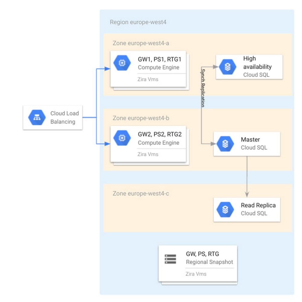
Editor’s note: In this blog, we look at how TIM Group, a leading information and communication technology (ICT) company in Italy and Brazil, used Cloud SQL for PostgreSQL to deliver a new billing application and saw 45% savings in database maintenance and infrastructure costs.In early 2020, TIM Group set out to solve a common challenge faced by large enterprises in order to keep up with competitive trends and new technological developments. One of our core IT systems, our billing function, was in need of a modernization overhaul and so we began a digital transformation project to build a new billing system on Google Cloud powered by Cloud SQL for PostgreSQL and Google Compute Engine. The new system was designed to automate important billing and credit systems that had been previously processed manually, and has already resulted in a 45% cost savings in database management, and a 20% savings in infrastructure costs. Designing a new digital journey My team is responsible for the development and maintenance of new billing systems for wholesale network access services. We began building a new system in 2020 that would modernize the way we bill for our B2B services with other telecom operators in the wholesale market, which in terms of revenue is an enormous market segment for TIM Group. The new billing system will help us to automate the formerly manual business processes for billing and credit management, and will eventually allow our IT department to decommission 16 legacy on-premise systems. Some of these legacy systems are 20 years old and no longer supported by the application stack. They suffer from poor performance, storage scalability limitations, low availability, and a lack of disaster recovery capabilities. In addition, they incur huge maintenance costs across applications and infrastructure levels, and they have no support for future use cases or innovation. Benchmarking Cloud SQL for a new billing systemWe initially started this project with a different planned architecture than the one we ended up building. At the outset, we had a blueprint architecture based on an Oracle database, and we acquired a license of a billing product called Wholesale Business Revenue Management (WBRM) from Zira to configure and customize as a base for our new billing system, compatible with both Oracle and PostgreSQL databases. Ultimately, we were designing a solution to run in our data centers based on VMware and Oracle, and a couple of months into the project we signed the partnership with Google Cloud. This decision opened up the possibility of running solutions on a modern cloud environment. We were excited by many of the capabilities we saw in Google Cloud’s solutions, including Cloud SQL, their fully managed relational database service for running MySQL, PostgreSQL and SQL Server. We tested the performance of Cloud SQL for PostgreSQL to see if it was comparable with the benchmark that Zira gave us for running WBRM on Oracle.The results were excellent; Cloud SQL for PostgreSQL met the Oracle database benchmark that Zira had given us based on previous stress tests. Using a database like Postgres would allow us to save on licensing costs and the contracting process with Oracle. To conduct these tests, we wanted to compare Oracle RAC against Cloud SQL for PostgreSQL, and look at which performed better in terms of application performance, scalability and ease of maintenance. We started with vertical scalability. We incremented the virtual CPUs and RAM by 20% and got a proportional benefit in throughput. We then tested horizontally scaled read workload and found that we had the same performance in user interface response time when linked to a read replica of a Cloud SQL for PostgreSQL database. We tested availability by switching down a node on the database, and found that all services were redirected to the follower node of the database with zero downtime. We were satisfied and encouraged by the results of these tests, and proceeded to build our new billing system with WBRM and Cloud SQL for PostgreSQL.Cutting database maintenance costs by up to 45%The managed services of Cloud SQL for PostgreSQL have given us considerable operational benefits. We were relying on external suppliers to handle most of our database maintenance, including updates, patching, security, and more administrative tasks. We saw 45% savings in eliminating that cost, and an additional 20% savings in infrastructure costs, which is a conservative estimate since we’re still in the process of fully rolling out the new system. We expect even bigger savings by the end of the project, which will hopefully go fully live at the end of 2021. Our project strategy has been to implement the new system in increments, replacing one service at a time. We started with services that weren’t supported by our legacy system, which included manual billing and credit processes that previously required 20-30 team members to maintain. As our year continues, we will continue work to dismiss legacy systems and to feed the new system with traffic usage, where we expect a huge ramp up of volume. Peeking under the hoodOur cloud instances are located primarily in the Netherlands region, with virtual machines in zones a and b for high availability. We have a highly available Cloud SQL instance across those zones. In zone c, we also have a read replica that we use to offload workloads from the primary that require read access only. For example, some departments have revenue assurance systems that connect to this read replica to check on orders billed or any revenue problems. On-premises, adding a new read replica server to the database can take two to three months, as it requires hardware allocation, tickets etc. In the cloud we can set up a read replica in a matter of minutes.For disaster recovery purposes, we make a daily backup with a 14 day retention period, and we have another operations team that is in charge of taking snapshots of our Zira VMs.Below, you can see our high level architecture. The application itself is hosted on Compute Engine and can be accessed through a load balancer. You can also see Cloud SQL and the read replicas in every zone and region mentioned above.Cloud SQL as part of the Zira WBRM architecture at TIM GroupTwo of our requirements were to direct some of the read traffic to the read replica and also to pool connections together. To meet those requirements, we have deployed PgBouncer which takes care of diverting the traffic and pgpool that takes care of connection pooling in front of Cloud SQL, as you can see in the diagram below.With Cloud SQL powering our new billing system, we can now automate previous manual billing and credit processing, dismiss over a dozen legacy systems, and build upon technology that provides high performance, easy storage scalability, high availability, and disaster recovery. And this is all at significant cost savings in database maintenance and infrastructure. In addition, we now have a database solution that integrates easily with other services like WBRM, and will empower TIM Group to innovate for use cases on our roadmap and beyond.Read more about TIM Group, Cloud SQL for PostgreSQL and Wholesale Business Revenue Management (WBRM) from Zira.Related ArticleIntroducing cross-region replica for Cloud SQLCross-region replication from Cloud SQL lets you ensure business continuity across Google Cloud regions in case of an outage or failure.Read Article
Quelle: Google Cloud Platform

How to load Salesforce data into BigQuery using a code-free approach powered by Cloud Data Fusion

Organizations are increasingly investing in modern cloud warehouses and data lake solutions to augment analytics environments and improve business decisions. The business value of such repositories increases as customer relationship data is loaded and additional insights are generated.In this post, we’ll cover different ways to incrementally move Salesforce data into BigQuery using the scalability and reliability of Google services, an intuitive drag-and-drop solution based on pre-built connectors, and the self-service model of a code-free data integration service. A Common Data Ingestion Pattern:To provide a little bit more context, here is an illustrative (and common) use case:Account, Lead and Contact Salesforce objects are frequently manipulated by call center agents when using the SalesForce application.Changes to these objects need to be identified and incrementally loaded into a data warehouse solution using either a batch or streaming approach.A fully managed and cloud-native enterprise data integration service is preferred for quickly building and managing code-free data pipelines.  Business performance dashboards are created by joining Salesforce and other related data available in the data warehouse.Cloud Data Fusion to the rescue To address the Salesforce ETL (extract, transform and load) scenario above, we will be demonstrating the usage of Cloud Data Fusion as the data integration tool. Data Fusion is a fully managed, cloud-native, enterprise data integration service for quickly building and managing code-free data pipelines. Data Fusion’s web UI allows organizations to build scalable data integration solutions to clean, prepare, blend, transfer, and transform data without having to manage the underlying infrastructure. Its integration with Google Cloud ensures data is immediately available for analysis. Data Fusion offers numerous pre-built plugins for both batch and real-time processing. These customizable modules can be used to extend Data Fusion’s native capabilities and are easily installed though the Data Fusion Hub component.For Salesforce source objects, the following pre-built plugins are generally available:Batch Single Source – Reads one sObject from Salesforce. The data can be read using SOQL queries (Salesforce Object Query Language queries) or using sObject names. You can pass incremental/range date filters and also specify primary key chunking parameters. Examples of sObjects are opportunities, contacts, accounts, leads, any custom object, etc. Batch Multi Source – Reads multiple sObjects from Salesforce. It should be used in conjunction with multi-sinks.Streaming Source – Tracks updates in Salesforce sObjects. Examples of sObjects are opportunities, contacts, accounts, leads, any custom object, etc.If none of these pre-built plugins fit your needs, you can always build your own by using Cloud Data Fusion’s plugin APIs. For this blog, we will leverage the out of the box Data Fusion plugins to demonstrate both batch and streaming Salesforce pipeline options.Batch incremental pipelineThere are many different ways to implement a batch incremental logic. The Salesforce batch multi source plugin has parameters such as “Last Modified After”, “Last Modified Before”, “Duration” and “Offset” which can be used to control the incremental loads.Here’s a look at a sample Data Fusion batch incremental pipeline for Salesforce objects Lead, Contact and Account. The pipeline uses the previous’ start/end time as the guide for incremental loads.Batch Incremental Pipeline – From Salesforce to BigQueryThe main steps of this sample pipeline are:For this custom pipeline, we decided to store start/end time in BigQuery and demonstrate different BigQuery plugins. When the pipeline starts, timestamps are stored on a user checkpoint table in BigQuery. This information is used to guide the subsequent runs and incremental logic.Using the BigQuery Argument Setter plugin, the pipeline reads from the BigQuery checkpoint table, fetching the minimum timestamp to read from.With the Batch Multi Source plugin, the objects lead, contact and account are read from Salesforce, using the minimum timestamp as a parameter passed to the plugin.BigQuery tables lead, contact and account are updated using the BigQuery Multi Table sink pluginThe checkpoint table is updated with the execution end time followed by an update to current_time column.Adventurous?You can exercise this sample Data Fusion pipeline in your development environment by downloading its definition file from GitHub and importing it through the Cloud Data Fusion Studio. After completing the import, adjust the plugin properties to reflect your own Salesforce environment. You will also need to:      Create a BigQuery dataset named from_salesforce_cdf_stagingCreate the sf_checkpoint BigQuery table on dataset from_salesforce_cdf_staging as described below:3. Insert the following record into the sf_checkpoint table:Attention: The initial last_completion date  = “1900-01-01T23:01:01Z” indicates the first pipeline execution will read all Salesforce records with LastModifedDate column greater than 1900-01-01. This is a sample value targeted for initial loads. Adjust the last_completion column as needed to reflect your environment and requirements for the initial run.After executing this sample pipeline a few times, observe how sf_checkpoint.last_completion column evolves as executions finish. You can also validate that changes are being loaded incrementally into BigQuery tables as shown below:BigQuery output – Salesforce incremental pipelineStreaming pipeline  When using the Streaming Source plugin with Data Fusion, changes in Salesforce sObjects are tracked using PushTopic events. The Data Fusion streaming source plugin can either create a Salesforce PushTopic for you, or use an existing one you defined previously using Salesforce tools. The PushTopic configuration defines the type of events (insert, update, delete) to trigger notifications, and the objects columns in scope. To learn more about Salesforce PushTopics, click here.   When streaming data, there is no need to create a checkpoint table in BigQuery as data gets replicated near real time, automatically capturing only changes, as soon as they occur. The Data Fusion pipeline becomes super simple as demonstrated in the sample below:Salesforce streaming pipeline with Cloud Data FusionThe main steps of this sample pipeline are:1. Add a Salesforce streaming source and provide its configuration details. For this exercise, only inserts and updates are being captured from CDFLeadUpdates PushTopic. As a reference, here is the code we used to pre-create the CDFLeadUpdates PushTopic in Salesforce. The Data Fusion plugin can also pre-create the PushTopic for you if preferred.Hint: In order to run this code block, login to Salesforce with the appropriate credentials and privileges, open the Developer Console and click on Debug | Open Execute Anonymous Window.2. Add a BigQuery sink to your pipeline in order to receive the streaming events. Notice the BigQuery table gets created automatically once the pipeline executes and the first change record is generated.After starting the pipeline, make some modifications to the Lead object in Salesforce and observe the changes flowing into BigQuery as exemplified below:BigQuery output – Salesforce streaming pipeline with Cloud Data FusionAdventurous?You can exercise this sample Data Fusion pipeline in your development environment by downloading its definition file from GitHub and importing it through the Cloud Data Fusion Studio. After completing the import, adjust the plugin properties to reflect your own Salesforce environment.Got deletes?  If your Salesforce implementation allows “hard deletes” and you must capture them, here is a non-exhaustive list of ideas to consider:An audit table to track the deletes. A database trigger, for example, can be used to populate a custom audit table. You can then use Data Fusion to load the delete records from the audit table and compare/update the final destination table in BigQuery.An additional Data Fusion job that reads the primary keys from the source and compare/merge with the data in BigQuery.A Salesforce PushTopic configured to capture delete/undelete events and a Data Fusion Streaming Source added to capture from the PushTopic.Salesforce Change Data Capture.Conclusion:If your enterprise is using Salesforce and If it’s your job to replicate data into a data warehouse then Cloud Data Fusion has what you need. And if you already use Google Cloud tools for curating a data lake with Cloud Storage, Dataproc, BigQuery and many others, then Data Fusion integrations make development and iteration fast and easy. Have a similar challenge? Try Google Cloud and this Cloud Data Fusion quickstart next. For a more in-depth look into Data Fusion check out the documentation.Have fun exploring!
Quelle: Google Cloud Platform

New Cloud Functions min instances reduces serverless cold starts

Cloud Functions, Google Cloud’s Function as a Service (FaaS) offering, is a lightweight compute platform for creating single-purpose, standalone functions that respond to events, without needing an administrator to manage a server or runtime environment. Over the past year we have shipped many new important capabilities on Cloud Functions: new runtimes (Java, .NET, Ruby, PHP), new regions (now up to 22), an enhanced user and developer experience, fine-grained security, and cost and scaling controls. But as we continue to expand the capabilities of Cloud Functions, the number-one friction point of FaaS is the “startup tax,” a.k.a. cold starts: if your function has been scaled down to zero, it can take a few seconds for it to initialize and start serving requests. Today, we’re excited to announce minimum (“min”) instances for Cloud Functions. By specifying a minimum number of instances of your application to keep online during periods of low demand, this new feature can dramatically improve performance for your serverless applications and workflows, minimizing your cold starts.Min instances in actionLet’s take a deeper look at min instances with a popular, real-world use case: recording, transforming and serving a podcast. When you record a podcast, you need to get the audio in the right format (mp3, wav), and then make the podcast accessible so that users can easily access, download and listen to it. It’s also important to make your podcast accessible to the widest audience possible including those with trouble hearing and those who would prefer to read the transcript of the podcast. In this post, we show a demo application that takes a recorded podcast, transcribes the audio, stores the text in Cloud Storage, and then emails an end user with a link to the transcribed file, both with and without min instances. Approach 1: Building the application with Cloud Functions and Cloud WorkflowsIn this approach, we use Cloud Functions and Google Cloud Workflows to chain together three individual cloud functions. The first function (transcribe) transcribes the podcast, the second function (store-transcription) consumes the result of the first function in the workflow and stores it in Cloud Storage, and the third function (send-email) is triggered by Cloud Storage when the transcribed result is stored and sends an email to the user to inform them that the workflow is complete.Fig 1. Transcribe Podcast Serverless WorkflowCloud Workflows executes the functions in the right order and can be extended to add additional steps in the workflow in the future. While the architecture in this approach is simple, extensible and easy to understand, the cold start problem remains, impacting end-to-end latency. Approach 2: Building the application with Cloud Functions, Cloud Workflows and min instancesIn this approach, we follow all the same steps as in Approach 1, with a slightly modified configuration that enables a set of min instances for each of the functions in the given workflow.Fig 2. Transcribe Podcast Serverless Workflow (Min Instances)This approach presents the best of both worlds. It has the simplicity and elegance of wiring up the application architecture using Cloud Workflows and Cloud Functions. Further, each of the functions in this architecture leverages a set of min instances to mitigate the cold-start problem and time to transcribe the podcast.Comparison of cold start performanceNow consider executing the Podcast transcription workflow using Approach 1, where no min instances are set on the functions that make up the app. Here is an instance of this run with a snapshot of the log entries. The start and end timestamps are highlighted to show the execution of the run. You can see here that the total runtime in Approach 1 took 17 s. Approach 1: Execution Time (without Min Instances)Now consider executing the podcast transformation workflow using Approach 2, where min instances are set on the functions. Here is an instance of this run with a snapshot of the log entries. The start and end timestamps are highlighted to show the execution of the run, for a total of 6 s. Approach 2: Execution Time (with Min Instances)That’s an 11 second difference between the two approaches. The example set of functions are hardcoded with a 2 to 3 second sleep during function initialization, and when combined with average platform cold-start times, you can clearly see the cost of not using min instances.You can reproduce the above experiment in your own environment using the tutorial here. Check out min instances on Cloud FunctionsWe are super excited to ship min instances on Cloud Functions, which will allow you to run more latency-sensitive applications such as podcast transcription workflows in the serverless model. You can also learn more about Cloud Functions and Cloud Workflows in the following Quickstarts: Cloud Functions, Cloud Workflows.Related ArticleRegistration is open for Google Cloud Next: October 12–14Register now for Google Cloud Next on October 12–14, 2021Read Article
Quelle: Google Cloud Platform

Protecting Healthcare data with DLP: A guide for getting started

Protecting patient data is of paramount importance to any healthcare provider. This is not only because of the many laws and regulations in different countries around the world requiring this data to be safeguarded, but it is a foundational requirement for trust between a provider and their patient. This does create some tension between patients and their providers.  To give patients the best care possible, a significant amount of Protected Health Information (PHI) is shared with providers who in turn share it with other providers, insurers, labs, etc. While sharing data can lead to better quality of care, it also introduces more risk to patient privacy.With many healthcare providers and insurers leveraging cloud technologies, the concerns around protecting PHI evolve. The various data types encountered in the healthcare ecosystem are diverse and complex, which means there are many different systems and formats to protect. This is where Cloud Data Loss Prevention (DLP) comes into play. Cloud DLP can help identify PHI/PII and help to obfuscate it, allowing for use of that data while adding additional layers of protection for the privacy of the patient.  This additional layer of protection compliments traditional security measures like access control, encryption-at-rest and encryption-in-transit by adding a layer of protection that can change or mask the data itself. This helps attain a deeper level of “least privilege” access, or data minimization. At Google Cloud we help many healthcare providers build and deploy globally scaled data infrastructure. These providers use Cloud Data Loss Prevention to discover PHI and protect it.In this series of articles, our goal is to discuss the various types of data formats (i.e. structured data, csv, etc) and systems in Google Cloud that may handle PHI and how the Google DLP API can be used across all of them to protect sensitive data.What is DLP?Cloud DLP helps customers inspect and mask this sensitive data with techniques like redaction, bucketing, date-shifting, and tokenization, which help strike the balance between risk and utility. This is especially crucial when dealing with unstructured or free-text workloads, in which it can be challenging to know what data to redact. Google Cloud DLP provides many system- and storage-agnostic capabilities that enable it to be used in virtually any workload, migration, or real-time application. In 2021, Forrester Research has named Google Cloud a Leader in The Forrester Wave™: Unstructured Data Security Platforms, Q2 2021 report, and rated Google Cloud highest in the current offering category among the providers evaluated. Additionally Cloud received the highest possible score in the Obfuscation criteria, a technique that can help protect sensitive data, like personally identifiable information (PII). While there are many great articles describing Google Cloud DLP and its components, for the purposes of this article we will focus on the key features of Cloud DLP that Healthcare providers leverage including:Data discovery and classificationData masking and obfuscationMeasuring re-identification risk Types of Data Healthcare Providers ManageWhile all Healthcare providers have data needs that are unique to their organization, we generally see Healthcare data falling into two buckets:Text-based dataThis data is typically seen as CSVs, flat files and transactional database entriesHL7/FHIR/DICOM dataThis data is typically received from EMR and other systems that follow interoperability standards in HealthcareIn the case of HL7/FHIR data the data is typically formed as a JSON or XML objectDICOM, being the standard for medical imaging, stores image files that often have text embedded in themThese common Healthcare data structures leverage various data sources and sinks to ingest, store and analyze data. The following is the list of the services we typically see leveraged for Healthcare data:Google Cloud StorageGoogle BigQueryGoogle Cloud SQLGoogle Cloud Pub/SubGoogle Cloud DataflowOne service in Google Cloud deserves a special callout here due to its impact on managing and leveraging Healthcare data and that is the Google Healthcare API. Check out overview videos and documentation here for more complete information on the Google Healthcare API. For the purposes of these articles we will focus on a few of its key capabilities including:Ingestion of HL7/FHIR dataIngestion of DICOM dataLeveraging DLP through the inbuilt features of the Healthcare APIGetting Started with DLP for Healthcare DataThere are a few key steps required to begin leveraging the DLP API which we will walk through. We will begin with a simple use case that scans a Google Cloud Storage bucket for the information we define, and replaces the information with the name of the information type. This is a good method to use to periodically scan a common data store for PHI, for example, in development environments.Inspecting DataThe first step is to create a template to instruct the DLP API on what data you need to find. To do so you will build an inspect template (example shown below). Inspect templates have many built-in infotypes (over 150) that allow users to discover common data elements that require redaction, like names, social security numbers, etc. It also allows for custom data types to be built in case you need to extend past the built-in detectors.Knowing where sensitive data exists is a critical step to protecting it. Using Cloud DLP to help discover, inspect, and classify data can help you understand how to best protect and secure your data. This inspection can be integrated into workflows to proactively detect and prevent data loss, or it can be used for ongoing inspections, which can generate security notifications/alerts when data is found in areas that it’s not expected. For the purposes of this article, we will show how to build an inspect template similar to the one that has been integrated into our Cloud Healthcare API for the de-identification of FHIR data, with a couple additional infotypes we often see used by our customers. There are many other built-in infotypes that are useful for Healthcare, like ICD10 codes.  We also added in a custom infotype to show how any regex can be used to match data based on unique needs.De-Identifying DataThe next step, de-identification, tells the DLP API what to do once it finds information based on the inspect template that you built. The De-Identify template can do many things such as:Tokenization with secure one-way hashingTokenization with two-way Deterministic Encryption or Format Preserving EncryptionDate shiftingData maskingBucketing or generalizationCombinations and variations of the aboveFor the purposes of this article we created a De-Identify template (shown below) that redacts the data matching the inspection configuration with the name of the infotype detected (i.e. [DATE_OF_BIRTH]). Many more options for what the De-Identify template can do can be found here.Scheduled Inspection JobsNow that you know what you are scanning for and the actions you want to take when sensitive data is discovered, you can schedule a scan. This process is well-documented here but these are a few key callouts before we proceed: When configuring a scan you must know the GCS bucket (or BigQuery dataset) that you want to scanWhen configuring your scan, consider reducing the sampling rate (percentage of data scanned) and only scanning data changed since the last scan to reduce costsWhile configuring the scan you will be given several options for notifications and outputs of DLP scans called Actions (seen below)These actions have various capabilities for analysis and notifications. Detailed descriptions of the options are listed here:Publish to BigQuery – This setting allows you to publish all results of DLP scans to a BigQuery dataset for future analysisPublish to Pub/Sub: This option will create messages in a selected Pub/Sub topic about the outcome of DLP scans. This is a great option if you want to have other applications, like a SIEM, consume the results.Publish to Security Command Center: Results can be published into Security Command Center for review by security teams.Publish to Data Catalog: If you leverage Data Catalog in your environment to manage and understand your data in Google Cloud, you can add your scan resultdata to your catalog.Notify by email: This action sends an email to project owners and editors when the job completes.Publish to Cloud Monitoring: Send inspection results to Cloud Monitoring in Google Cloud’s Operations suite.See ResultsIn the console, navigate to Data Loss Prevention and select the Inspection tab. You should see what is indicated in the following image:If you select any job ID you will see the job details including findings, bytes scanned, errors, and a result listing that shows which infotypes were discovered.As noted above, you can send your results to many locations via DLP Actions. Thanks to that flexibility, there are many options for bespoke solutions on current BI tools to analyze scan results. If you don’t have that tooling available, a great solution could be to send your results to BigQuery and use a Data Studio dashboard to analyze your results.Next StepsIn this article we started down the path of leveraging DLP to protect PHI in Healthcare environments. Now that we have the basic building blocks set up, we want to start using them.In the rest of this blog post series we will discuss:DLP use cases for the different data stores commonly used in HealthcareDLP in the Healthcare APIAlternate De-Identification methodsViewing and managing scanning resultsGoogle Cloud DLP is built for the modern technology landscape. By utilizing the steps above, you can create a secure foundation for protecting patient data. The Google Cloud team is here to help. To learn more about getting started on DLP or general best practices to manage risk, reach out to your Technical Account Manager or contact a Google Cloud account team.Related ArticleImproving security, compliance, and governance with cloud-based DLP data discoveryData discovery, a key component of DLP technology, has never been more important. Here’s why.Read Article
Quelle: Google Cloud Platform

Google Cloud VMware Engine, PowerCLI and BigQuery Analytics

Google Cloud Billing allows Billing Account Administrators to configure the export of Google Cloud billing data to a BigQuery dataset for analysis and intercompany billback scenarios. Developers may choose to extract Google Cloud VMware Engine (GCVE) configuration and utilization data and apply internal cost and pricing data to create custom reports to support GCVE resource billback scenarios.  Using VMware PowerCLI, a collection of modules for Windows PowerShell, data is extracted and loaded into Big Query. Once the data is loaded into Big Query, analysts may choose to create billing reports and dashboards using Looker or Google Sheets. Exporting data from Google Cloud billing data into a BigQuery dataset is relatively straight-forward. However, exporting data from GCVE into BigQuery requires PowerShell scripting. The following blog details steps to extract data from GCVE and load it into BigQuery for reporting and analysis. Initial Setup VMware PowerCLI InstallationInstalling and configuring VMware PowerCLI is a relatively quick process, with the primary dependency being network connectivity between the host used to develop and run the PowerShell script and the GCVE Private Cloud.[Option A] Provision a Google Compute Engine instance, for example Windows Server 2019, for use as a development server. [Option B] Alternatively, use a Windows laptop with Powershell 3.0 or higher installedLaunch the Powershell ISE as Administrator. Install and configure the VMware PowerCLI, any required dependencies and perform a connection test.Reference: https://www.powershellgallery.com/packages/VMware.PowerCLI/12.3.0.17860403 VMware PowerCLI DevelopmentNext, develop a script to extract and load data into BigQuery. Note that this requires a developer to have permissions to create a BigQuery dataset, create tables and insert data. An example process including code samples follows. 1. Import the PowerCLI Module and connect to the GVCE cluster.2. [Optional] If desired, a vCenter simulator docker container, nimmis/vcsim : vCenter and ESi API based simulator, may be useful for development purposes. For information on setting up a vCenter simulator, see the following link: https://www.altaro.com/vmware/powercli-scripting-vcsim/ 3. Create a dataset to hold data tables in BigQuery. This dataset may hold multiple tables. 4. Create a list of vCenters you would like to collect data from.5. Create a file name variable.6. For a simple VM inventory, extract data using the Get-VM cmdlet. You may also choose to extract data using other cmdlets, for example, Get-VMHost and Get-DataStore. Review vSphere developer documentation for more information on available cmdlets along with specific examples. 7. View/Validate the json data as required.8. Create a table in BigQuery. Note that this only needs to be done once. In the example below the .json file was first loaded into a Cloud Storage bucket. The table was then created from the file in the bucket.9. Load the file into Big Query.10. Disconnect from a server. 11. Consider scheduling the script you developed using Windows Task Scheduler, cron or another scheduling tool so that it runs on the required schedule.12. Using the BigQuery UI or Google Data Studio, create views and queries referencing the staging tables to extract and transform data for reporting and analysis purposes. It’s a good idea to create any supporting tables in BigQuery to support cost analysis such as a date dimension table, pricing schedule table and other relevant lookup tables to support allocations and departmental bill back scenarios. Connect to Big Query using Looker to create reports and dashboards. Example: Connect to BigQuery from Google Sheets and Import data.Using Custom TagsCustom tags allow a GCVE administrator to associate a VM with a specific service or application and are useful for bill back and cost allocation. For example, vm’s that have a custom tag populated with a service name (ex. x-callcenter) can be grouped together to calculate direct costs required to deliver a service.  Jump boxes or shared vm’s may be tagged accordingly and grouped to support shared service and indirect cost allocations.  Custom tags combined with key metrics such as provisioned, utilized and available capacity enable GCVE administrators to optimize infrastructure and support budgeting and accounting requirements. Serverless Billing Exports scheduled with Cloud SchedulerIn addition to running powershell code as a scheduled task, you may choose to host your script in a container and enable script execution using a web service. One possible solution could look something like this: Create a Docker File running ubuntu 18:04. Install Python3, Powershell 7  and VmWare Power CLIExample requirements.txtExample Docker File: 2. For your main.py script, use subprocess to run your powershell script.  Push your container to Container Registry , deploy your container and schedule ELT using Cloud Scheduler. Related ArticleGoogle Cloud VMware Engine explained: Integrated networking and connectivityLearn about the networking features in Google Cloud VMware Engine to let you easily and deploy workloads across on-prem and cloud environ…Read Article
Quelle: Google Cloud Platform

Anomaly detection with TensorFlow Probability and Vertex AI

Time series anomaly detection is currently a trending topic—statisticians are scrambling to recalibrate their models for retail demand forecasting and more given the recent drastic changes in consumer behavior. As an intern, I was given the task of creating a machine-learning based solution for anomaly detection on Vertex AI to automate these laborious processes of building time series models. In this article, you will get a glimpse into the kinds of hard problems Google interns are working on, learn more about TensorFlow Probability’s Structural Time Series APIs, and learn how to run jobs on Vertex Pipelines.Vertex PipelinesVertex Pipelines is Google Cloud’s MLOps solutions to help you “automate, monitor, and govern your ML systems by orchestrating your ML workflows.” More specifically, our demo runs on the open source Kubeflow Pipelines SDK that can run on services such as Vertex Pipelines, Amazon EKS, and Microsoft Azure AKS. In this article we demonstrate how to use Vertex Pipelines to automate the process of analyzing new time series data, flagging anomalies, and analyzing these results. To learn more about Vertex Pipelines, read this article.Google Cloud Pipeline ComponentsGoogle Cloud Pipeline Components is Kubeflow Pipeline’s new initiative to offer various solutions as components. Our time series anomaly detection component is the first applied ML component offered in this SDK. You can view our open source component in the SDK’s Github repo, and you can use the component by loading it via url.Note that the component is in experimental mode and has not yet been officially released.TensorFlow Probability Anomaly Detection APITensorFlow Probability has a library of APIs for Structural Time Series (STS), a class of Bayesian statistical models that decompose a time series into interpretable seasonal and trend components. Previously, users had to hand define the trend and seasonal components for their models, for example the demo uses a model with a local linear trend and month-of-year seasonal effect for CO2 concentration forecasting. In conjunction with this intern project, the TensorFlow Probability team built a new anomaly detection API where these components are inferred based on the input time series. This means that users can now do anomaly detection in one line of code:This end-to-end API regularizes the input time series, infers a seasonal model, fits the model, and flags anomalies based on the predictive bounds of acceptable values. It is currently available in the TensorFlow Probability Github repository and will be included in the next official release. Our Google Cloud Pipeline Component packages this API onto the Vertex Pipelines ecosystem and demonstrates an example workflow using this anomaly detection algorithm.Demo NotebookIn our demo, we benchmark the performance of the TensorFlow Probability anomaly detection algorithm on the NYC Taxi task from the Numenta Anomaly Benchmark. This dataset records the total number of NYC taxi passengers from July 2014 – January 2015 in 30-minute increments. There are ~10k data points and 5 anomalies that occur during events like Christmas and the NYC marathon.Here we visualize the results of our pipeline. In the top graph, the black line marks the original time series of taxi passengers over time. The blue distribution marks the forecast distribution that the algorithm deems as likely given the previous time points, meaning any point above or below the forecast is flagged as anomalous. In the bottom graph, the black boxes mark the residual, i.e. the difference between the observed and expected counts of passengers. Here we see that there is a high residual on December 25th and the algorithm correctly flags the day as an anomaly.We also run the custom scoring script from the Numenta Anomaly Benchmark on our predictions to compare the algorithm with others. We see that our algorithm performs the best on this NYC Taxi task as it is able to detect more anomalies with minimal false positives.ConclusionWant to start building your own time series models on Vertex AI? Check out the resources below to dive in:Colab notebook for time series anomaly detectionDocumentation on building your first KFP componentTensorFlow Probability blog post on Structural Time Series ModelingTensorFlow Probability demo for Structural Time Series Modeling Case StudiesRelated ArticleBuild a reinforcement learning recommendation application using Vertex AIIn this article, we’ll demonstrate an RL-based movie recommender system, including a MLOps pipeline, built with Vertex AI and TF-Agents.Read Article
Quelle: Google Cloud Platform

Real-time analytics made easy with Cloud Spanner federated queries with BigQuery

As enterprises compete for market share, their need for real-time insights has given rise to increased demand for transactional databases to support data analytics. Whether it’s to provide dashboards that inform rapid decision-making, to perform analysis on a lookup table stored in a transactional database, or to conduct complex hybrid transactional analytical workloads, there is a growing demand for analyzing large volumes of data in transactional databases.Cloud Spanner is Google Cloud’s fully managed relational database for transactional workloads, and today, with the general availability of Spanner federated queries with BigQuery, it gets even more powerful. BigQuery is Google Cloud’s market-leading serverless, highly scalable, multi-cloud data warehouse that makes analytics easy by bringing together data from multiple sources. With Spanner’s BigQuery federation, you can query data residing in Spanner in real time without moving or copying the data, bridging the gap between operational data and analytics and creating a unified data lifecycle.It’s already been possible to use tools like Dataflow to copy data from Spanner over to BigQuery, but if you haven’t set up these ETL workflows — or you simply need to do a quick lookup on data that’s in Spanner — you can now take advantage of BigQuery’s query federation support to run real-time queries on data that’s stored in Spanner. In this post, we’ll look at how to set up a federated query in BigQuery that accesses data stored in Spanner.How to run a federated querySuppose you’re an online retailer that uses Spanner to store your shopping transactions, and you have a Customer 360 application built in BigQuery. You can now use federated queries to include this customer’s shopping transactions in your Customer 360 application without needing to copy the data over to BigQuery from Spanner.To run a Customer 360 query in BigQuery that includes the shopping transactions that are stored in Spanner, follow these steps:Launch BigQuery and choose the Google Cloud project that contains the Spanner instance that includes the shopping transactions database.Set up an external data source for the Spanner shopping database in BigQuery. You’ll need to have bigquery.admin permissions to set this up.Write a query in BigQuery that accesses the shopping data in the Spanner data source. If you’d like other users to access this external data source in BigQuery, simply grant them permission to use the connection resource you just created.Setting up an external data sourceTo setup a Spanner external data source, select “Add data” and choose “External Data Source”From here, add the connection settings for your Spanner database.Writing a query that accesses the Spanner data sourceOnce you’ve created the external data source, it will be listed as one of the external connections in your project in the BigQuery Explorer.Now, you simply use the EXTERNAL_QUERY function to send a query statement to Spanner, using Spanner’s native SQL dialect. The results are converted to BigQuery standard SQL data types and can be joined with other data in BigQuery.Here’s the syntax for using EXTERNAL_QUERY:SELECT * FROM EXTERNAL_QUERY(connection_id, external_database_query);Connection_id(string): The name of the Spanner database connection resource. It is of the form: projects/projectID/locations/us/connections/ConnectionID. ConnectionID is the connection ID you created when you set up the external data source.external_database_query (string): a read-only query in Spanner’s SQL dialect. The query is executed in Spanner and returned as a table in BigQuery.For example:And it’s as simple as that. There’s no need to copy data from Spanner over to BigQuery — EXTERNAL_QUERY takes care of everything. Moreover, EXTERNAL_QUERY returns a table that is no different from any other table in BigQuery, so you can JOIN to it, add it to materialized and authorized views, populate a dashboard with it, and even schedule the query using BigQuery’s scheduler.Advantages of using Spanner federated queries with BigQuery When you use query federation, the query is run by Spanner, and the results are returned to BigQuery as a table. The data is accessed in real-time; there’s no need to wait for an ETL job to complete for the freshest of data.The query will be executed by Spanner, so you’ll be able to take advantage of the same query optimizer and SQL capabilities that you’ll find in Spanner. You’ll also have the option to take advantage of Spanner’s PartitionQuery capabilities. You’ll likely find EXTERNAL_QUERY is useful for lookups and simple analytics in Spanner tables rather than intensive analytics that would benefit from BigQuery’s strong analytic capabilities. For more intensive analytics, you can still use EXTERNAL_QUERY to copy the data over to BigQuery rather than writing ETL jobs, and continue to run the analytics in BigQuery, such as the following:Learn moreTo get started with Spanner, create an instanceor try it out with a Spanner Qwik Start.To learn more about Spanner federated queries with BigQuery, see the documentation.Related ArticleRegistration is open for Google Cloud Next: October 12–14Register now for Google Cloud Next on October 12–14, 2021Read Article
Quelle: Google Cloud Platform

Replicating from Cloud Spanner to BigQuery at scale

Cloud Spanner is GCP’s native and distributed Online Transaction Processing System (OLTP). Due to its distributed nature, it can scale horizontally and therefore is suitable for workloads with very high throughputs containing large volumes of data. This invites a huge opportunity to do analytics on top of it. Thanks to Cloud Spanner BigQuery Federation, you can now easily fetch Cloud Spanner data into BigQuery for analytics. In this post, you will learn how to efficiently use this feature to replicate large tables with high throughput (lots of inserts or updates written per second), with low to medium replication lag.ELT process optimizationsSetting up an efficient Extract Load and Transform (ELT) to fetch data from Cloud Spanner to BigQuery is the key for low replication lag. After performing an initial full load, you will need to set up incremental loads. For large tables in Cloud Spanner, refreshing full data every time can be slow and costly. Therefore it is more efficient to extract only new changes and merge with existing data in BigQuery.Designing Cloud Spanner for incremental dataTaking an example table schema such as below:In order to identify incremental changes, you will need to add a commit timestamp column (say lastUpdateTime). In addition, your application will need to pass PENDING_COMMIT_TIMESTAMP(), so that Cloud Spanner updates the corresponding field post commit.To efficiently read the rows changed after a certain timestamp you will need to create an index. Since indexes on monotonically increasing values can cause hotspots you will need to add another column (say shardid) and create a composite index using (shardid, lastUpdatedTime). Updated schema would look as below:In the above example, I have added LastUpdateTime as a commit timestamp column. Also added ShardId as a generated column which will produce values in range of -18 to +18. This helps in avoiding hotspots when indexing timestamp by creating composite an index on (ShardId, LastUpdateTime). Further you can make it a NULL FILTERED index to keep it light. You can periodically update LastUpdateTime as null for old records. Read here for a more detailed solution.Now to query incremental changes from the table SQL query will be as follows:Above sql query reads data from all shards as well as filters on LastUpdateTime. Therefore using the index to optimize reading speed from large tables.Initial loading of data into BigQueryLoading data for the first time is likely to read the entire table in Cloud Spanner and send results into BigQuery. Therefore you should create a connection with the “Read Data in Parallel” option.Below is an example sql query to do the initial load.Incrementally loading data into BigQueryUpdate the connection (or create new connection) with “Read data in parallel” unchecked.This is because (at the time of writing), Spanner queries using indices are not root partitionable and the result cannot be read in parallel. This might get changed in future.After getting incremental data from Cloud Spanner it should be stored into a staging table in BigQuery, thus completing the Extract and Load part of (ELT). Finally you will need to write a Merge statement to consolidate incremental data into a BigQuery table.Thanks to BigQuery’s scripting all of this ELT can be combined into a single script as below and further it can be configured as scheduled query.Above script finds last time bigquery was updated for that table. It constructs a SQL Query to fetch any incremental data post last fetch and store it as a staging table. Then merge new data into bigquery table and finally delete the staging table. Explicit dropping of table ensures that two parallel executions of above script will fail. This is important so that if there is a sudden surge then no data shall be missed.Other considerationsCreating table partitions in BigQueryIt is common to create table partitions and clustering based on your reads / analytics requirements. However, this can lead to a low merge performance. You should make use of BigQuery partitioning and clustering in such cases.Clustering can improve match performance, therefore you can add clustering on the PK of the table. Merging data rewrites entire partitions, having partition filters can limit volume of data rewritten. Handling deleted rowsAbove solution will skip over deleted rows, which might be acceptable for many use-cases. However if you need to track the deletes then the application will need to implement soft deletes like add a column isDeleted = true/false. Data from Cloud Spanner should be hard deleted after some delay so that changes are synchronized into BigQuery first.During merge operation in bigquery you can conditionally delete based on the above flag.What’s nextIn this article you learned about how to replicate data from Cloud Spanner to BigQuery. If you want to test this in action, use Measure Cloud Spanner performance using JMeter for a step by step guide on generating sample data on Cloud Spanner for your workload schema.Related ArticleMeasuring Cloud Spanner performance for your workloadIn this post, we will explore a middle ground to performance testing using JMeter. Performance test Cloud Spanner for a custom workload b…Read Article
Quelle: Google Cloud Platform

All you need to know about Cloud Storage

Cloud Storage is a global, secure, and scalable object store for immutable data such as images, text, videos, and other file formats. You can add data to it or retrieve data from it as often as your application needs. The objects stored have an ID, metadata, attributes, and the actual data. The metadata can include all sorts of things,  including the security classification of the file, the applications that can access it, and similar information. The ID, metadata, and attributes make object storage an appealing storage choice for a large variety of applications ranging from web serving to data analytics. Click to enlargeStorage classesYou store objects in buckets that are associated with a project, which are, in turn, grouped under an organization. There are four storage classes that are based on budget, availability, and access frequency. Standard buckets for high-performance, frequent access, and highest availabilityRegional or dual-regional locations for data accessed frequently or high-throughput needsMulti-region for serving content globallyNearline for data accessed less than once a month Coldline for data accessed roughly less than once a quarterArchive for data that you want to put away for years (accessed less than once a year)It costs a bit more to use standard storage because it is designed for short-lived and/or frequently accessed data. Nearline, coldline, and archive storage offer a lower monthly storage cost for longer-lived and less frequently accessed data. Choosing a location for your use caseCloud Storage lets you store your data in three types of locations:Regional: all of your data is stored redundantly in a single region. Regional buckets usually offer the lowest monthly storage price and are suitable for a wide range of use cases, including high-performance analytics where it is important to co-locate your compute and storage in the same region.Multi-region: all of your data is stored redundantly across a continent but it’s not visible which specific regions your data is in. Availability is higher than regional because your data can be served from more than one region. Multi-regions cost a little more than single regions, but are great choices for content serving to the Internet.Dual-regions: all of your data is stored in two specific regions. Dual-regions provide the best of regions and multi-regions — providing you with high availability and protection against regional failures while also giving you the high-performance characteristics of regional storage. Business-critical workloads are often best implemented on top of dual-regions. Dual-regions can also be a great choice for a data lake for streaming as well as for batch uploading of data for big data and ML projects.No matter the location that you select, all four storage classes are available to you so that you can optimize your costs over time, storing your most active “hot” data in Standard and moving it down to colder classes as it becomes older and less frequently accessed.How to use Cloud Storage With Object Lifecycle Management you can automatically transition your data to lower-cost storage classes when it reaches a certain age or when other lifecycle rules that you’ve set up apply. Cloud Storage also offers automatic object versioning, so you can restore older versions of objects—which can be especially helpful as protection against accidental deletion.You can upload objects to the bucket and download objects from it using the console or gsutilcommands, Storage Transfer Service, Transfer Appliance, or transfer online. Once you have stored the data, accessing it is easy with a single API call for all storage classes. For a more in depth look at optimizing location and costs for your Cloud Storage buckets, check out this article: Optimizing object storage costs in Google Cloud: location and classes.SecurityBy default 100% of data in Cloud Storage is automatically encrypted at rest and in transit with no configuration required by customers. You can grant permission to specific members and teams or make the objects fully public for use cases such as websites.If you want more direct control over encryption you have two additional key management options available to you that go beyond the built-in encryption that Google manages for you: You can use customer-managed encryption keys (CMEK) via Google Cloud Key Management Service (KMS). You can define access controls to encryption keys, establish rotation policies, and gather additional logging into encryption/decryption activities. In both the default and customer-managed case, Google remains the root of trust for encryption/decryption activities. You can use customer-supplied encryption keys (CSEK) in which Google is no longer in the root of trust. Using CSEK comes with some additional risk of data loss, as Google cannot help you decrypt data if you lose your encryption keys.Furthermore, you do not have to choose one key management option only. You can make use of the default encryption for most of your workloads, and add some extra control for select applications.ConclusionWhether you need to store data for regulatory compliance, disaster recovery, analytics, or simply serving it on the web, Cloud Storage has you covered. For a more in-depth look check out the Cloud Storage Bytes video series. For more #GCPSketchnote, follow the GitHub repo. For similar cloud content follow me on Twitter @pvergadia and keep an eye out on thecloudgirl.dev.
Quelle: Google Cloud Platform

Six new features in Dialogflow CX

Today, we are excited to announce the public preview of six new features in Dialogflow CX that make it the best chatbot virtual agent for enterprises.With these features, our customers will be able to improve the end-user conversational experience and manage security and deployment better. These launches also include some console improvements and built-in support for making the bot building experience more efficient.Here’s a selection of what’s new:Streaming partial responsePrivate network access to Webhook targetsSearch in consoleSystem functions supportContinuous tests and deploymentChange Diffs in Change HistoryStreaming Partial ResponseUntil now, Dialogflow CX was only able to send ordered responses to the end user once the agent’s turn was over (which includes webhook execution). For some customers, it can take 10-15 seconds for their webhooks to execute, during which time, the bot is silent and the end user is left waiting (and probably wondering!)Owing to the Streaming Partial Response feature, if a webhook will likely run for a long time, customers can now add a static response in the fulfillment and enable partial response when using streaming APIs. This way, the Dialogflow Streaming API will send partial bot responses to the user while the webhook is executing, improving the ‘perceived’ latency in such scenarios. Here’s a sample conversation without partial response:Now, a sample conversation with partial response:To enable partial response use the toggle button under the ‘Fulfillment’ section in the Dialogflow CX UI as shown below:Private network access to Webhook targets  Dialogflow now integrates withService Directory private network access so it can connect to webhook targets inside our customers’ VPC network. This keeps the traffic within the Google Cloud network and enforcesIAM andVPC Service Controls for enterprise security. Learn more about setting this up in our Dialogflow CX documentation.Search EverywhereWondering how to navigate through hundreds of intents, thousands of training phrases? Dialogflow CX’s new global search functionality enables users to search, filter and access  resources like pages, intents, training phrases, entity types, webhooks, route groups and more. One can easily search relevant resources using the ‘resource type’ filter while searching. Search results can further be narrowed down by clicking on the ‘Search Options’ icon. This allows users to specify a criteria for filtering search results. For instance, users can search for intents containing a certain training phrase, routes referencing a certain intent and more. Continuous Tests and DeploymentBuilding an enterprise-grade bot often involves intensive QA (Quality Assurance) and deployment processes, which can lead to a lot of manual work. The CI/CD (Continuous Integration/Continuous Deployment) feature in Dialogflow CX aims to assist bot developers with new tools to manage their bot release cycles.Using this feature, one can automatically run a set of test cases configured for an environment to verify the intended behavior of the agent in that environment. Users can also use the continuous deployment setting to run verification tests before deploying a flow version to the environment to prevent unintended behaviors and minimize errors.System functionsDialogflow now has supportedsystem functions that can execute common arithmetic, string manipulation, conditional and date/time operations. This will save our users the extra effort to write code for these operations, thus improving efficiency. This is also a step towards centralization of business logic of the bot, reducing dependency on webhooks. Customers can apply these inline system functions in their agent’sconditions and fulfillments (such astext responses,conditional responses andparameter presets) to generate dynamic values during conversations. Here’s an example:Here the agent is responding back with a dynamically calculated count of the number of items in a customer’s list. The dynamic calculation is made possible by simply using system functions for counting the number of parameters (COUNT) in the session and converting that number to text (TO_TEXT) for display. CurrentFunctions list:Arithmetic operations: ADD, MINUS, RANDString manipulation: LOWER, SUBSTITUTE, SPLIT, JOIN, CONCATENATE, MID, LEN, TO_TEXT, CONTAINConditional: IFDate/time: NOW, FORMAT_DATEOther: COUNTChange DiffsDialogflow CX makes it really easy to work with teams on a single agent, with this new enhancement to the Change history feature in Dialogflow CX, which logs changes made to the agent. Users can now click each entry in the change history table to view the before and after of each resource and see exactly what changed.Sample screenshot:ConclusionWith these new features in Dialogflow CX, it is easier for enterprises to build and manage large and complex agents. Streaming partial responses will improve the experience of the end user when connecting to external systems via webhooks. The search functionality and system functions will help make the bot building process more efficient. The features around continuous tests and deployment will make it easier to manage the CI/CD pipeline. And with the Service Directory integration for private network access in webhooks, enterprises can better secure their back-end code. Finally, change diffs along with change history will make change management easier while working with large teams.Stay tuned for more features that will enhance the collaboration experience in Dialogflow CX, visual builder improvements and features to help our power users build and manage bots more efficiently.Related ArticleRespond to customers faster and more accurately with Dialogflow CXNew Dialogflow CX Virtual Agents can jumpstart your contact center operational efficiency goals, drive CSAT up and take care of your huma…Read Article
Quelle: Google Cloud Platform