Cloud Computing Köln - Seite 3532 von 7138 - Neues zu Cloud Computing, Internet of Things und Technologien

In part one of the series, we discussed how the Red Hat OpenShift Scale-CI evolved. In part two of the series, we looked at the deep dive and various components of Scale-CI. In this post, we will look at the highlights of how we used OpenShift Scale-CI to test and push the limits of OpenShift 4.1 which is the first OpenShift 4.x release and OpenShift 4.2 at scale.
We typically use hardware resources from the scale lab, a datacenter built and managed by Red Hat’s Performance and Scale team with the goal to provide compute resources on demand to various teams across Red Hat to solve problems related to Performance and Scalability. We install OpenStack on the bare metal machines to manage the resources and then install OpenShift on the virtual machines. In OpenShift 3.x, the installer doesn’t take care of provisioning which means that we need to build wrapper scripts to create virtual machines for installing and scaling up OpenShift whereas the OpenShift 4.x IPI (Installer Provisioned Infrastructure) based installer takes care of provisioning and scaling up the cluster to higher node counts literally takes minutes versus hours. Redhat Enterprise Linux CoreOS is the default base operating system for OpenShift 4.x, It is immutable which means that configurations and packages can’t be changed or installed on the host, everything needs to run as a container. The cluster has full control over the nodes, this will avoid configuration drifts leading to easier upgrades and achieves repeatability and auditability. The following diagram shows the fully automated day 1 and day 2 operations:

A single blog post won’t be sufficient to elaborate on the amazing features and enhancements including the operators, you can refer to the 4.1 release notes and 4.2 release notes to know about all the features.
Let’s jump straight into the OpenShift 4.1 and 4.2 scale test run highlights. We picked AWS and GCP as the cloud platforms to host OpenShift 4.1 and 4.2 clusters respectively. AWS is the only supported provider ( Installer Provisioned Infrastructure ) for the OpenShift 4.1 release while GCP, Azure and Red Hat OpenStack Platform are also supported in OpenShift 4.2. Here is the cluster configuration:

The 4.1 and 4.2 clusters consisted of 3 Masters/Etcd with io1 and SSD storage in the case of AWS and GCP respectively, etcd is i/o intensive especially when the cluster consists of large number of nodes and objects. We create infrastructure nodes using custom machinesets as part of day 2 operation to host prometheus, router, registry and logging instead of using bigger worker nodes and setting the limits on the deployments for the infrastructure components to be scheduled on nodes with the available resources.
We ran a bunch of scale tests including:

Kubelet density focused test which spawns maximum pods across the worker nodes which is 250 ( current cluster limits for OpenShift 4.1 and 4.2 ).
Control plane density focused tests which creates a bunch of projects with secrets, configmaps, routes, builds, deployments e.t.c across the cluster to stress the apiserver, etcd and controller on masters/etcd nodes.
HTTP/Router scale test, a data-plane workload generator that runs http requests through through HAProxy into deployed pods.
Cluster Limits, we ran a bunch of tests to validate and push the limits for the OpenShift 4.1 and 4.2 releases. The findings have been documented as part of the Scalability and Performance guide to help users/customers plan their environment according to the object limits. The following table shows the cluster limits for various OpenShift releases:

Networking scale tests which runs uperf benchmarks testing node to node, pod to pod, and svc to svc throughput and latency for TCP and UDP protocols.

We also ran scale tests focusing on Monitoring ( Prometheus ), Logging ( Fluentd and Elasticsearch ), Storage and Registry. The scale tests are all hosted in workloads and svt repositories and are triggered using the pipeline. Here are some of the interesting findings, tunings and recommendations from the runs:

Etcd is a critical component of OpenShift, It stores and replicates the cluster state.

For large and dense clusters, etcd can suffer from poor performance if the keyspace grows excessively large and exceeds the space quota. Periodic maintenance of etcd including defragmentation needs to be done to free up space in the data store. It is highly recommended that we monitor Prometheus for etcd metrics and defragment it when needed before etcd raises a cluster-wide alarm that puts the cluster into a maintenance mode, which only accepts key reads and deletes. Some of the key metrics to monitor are etcd_server_quota_backend_bytes which is the current quota limit, etcd_mvcc_db_total_size_in_use_in_bytes which indicates the actual database usage after a history compaction, and etcd_debugging_mvcc_db_total_size_in_bytes which shows the database size including free space waiting for defragmentation. The default Etcd space quota is 7GB, it should be good enough to support large and dense clusters. Etcd maintenance is a day 2 operation as the defragmentation is not done automatically, it is essential to monitor the metrics mentioned and act accordingly.

Some users have requirements especially when running OpenShift on bare metal nodes might not have the luxury to use thousands of nodes in case they want to run thousands of pods. This motivated us to work on pushing the pods per node limit beyond the current supported limit of 250 pods per node – the work is still in progress.
Scaling up the cluster to higher node counts is as simple as changing the replica count of the worker machinesets. The worker nodes are distributed across various zones of a region in the public cloud ( AWS and GCP in our case ), it’s recommended to spread them across the availability zones evenly during the scaleup as well for higher availability.
We ran baseline workload to collect data on a base cluster with no applications running except the system components. As we keep adding enhancements to make OpenShift self healing/managed by operators, support over the air upgrades to make our life easy and also have a better user experience, the number of containers/components which run by default on the cluster increased when compared to OpenShift 3.x. The document has details about the recommended master node sizes for various node scale.
ROUTER_THREADS is 4 by default in OpenShift 4.x, the router performance optimizations have been documented as part of the OpenShift Scalability and Performance Guide.
The new fluentd version 1.2.x used in OpenShift 4.1 and 4.2 provides over twice the single node message throughput as the version used in OpenShift 3.x.
The Elasticsearch version used in OpenShift 4.1 and 4.2 is unchanged from OpenShift 3.11 and message indexing throughput is comparable to that release.
Source-to-image (S2I) build times in OpenShift 4.1 were longer than previous releases for several reasons related to how s2i builds are run and pushed to the internal registry. In OpenShift 4.2, the times were improved by 2x – 3x.
There might be a need to tweak the kubelet config for example the qps/burst rates or the pods per node, it takes hours for the change to take effect on a cluster with large number of nodes as the change triggers a reboot of the nodes to apply the configuration and the number of nodes which can be unavailable at a given time by default is 1, it can be tweaked to speed up the process as documented in the Scalability and Performance Guide.

NOTE: When setting the value, consider the number of worker nodes that can be unavailable without affecting the applications running on the cluster.

We ran tests focusing on Cluster Monitoring Operator to come up with the Prometheus Database storage requirements based on number of nodes/pods in the cluster, the recommendations have been documented as part of the OpenShift Scalability and Performance Guide.
The rate at which the kubelet talks to the API server depends on queries per second (QPS) and burst values. The default values, 5 for kubeAPIQPS and 10 for kubeAPIBurst, are good enough if there are limited pods running on each node. Updating the kubelet QPS and burst rates is recommended when there are a large number of objects provided there are enough CPU and memory resources on the node, the information on how to tweak the values is discussed in the guide.
Scaling pods with attached PVC was very reliable and consistent with only limitation being the imposition by the public cloud providers on the number of block devices per cloud instance.
The upgrades got much easier and reliable. The machine-config operator will start complaining during the upgrades even if a single file/config is changed on the host.

Look out for part 4: Tooling/Automation Enhancements and Highlights of OpenShift 4.3 Scale Test Run. As always, feel free to reach us on sig-scalability kubernetes slack or on github. Any feedback and contributions are most welcome.
The post OpenShift Scale-CI: Part 3 – OCP 4.1 and 4.2 Scale Run Highlights appeared first on Red Hat OpenShift Blog.
Quelle: OpenShift

12. Dezember 2019

da Agency

Combine the Power of Video Indexer and Computer Vision

We are pleased to introduce the ability to export high-resolution keyframes from Azure Media Service’s Video Indexer. Whereas keyframes were previously exported in reduced resolution compared to the source video, high resolution keyframes extraction gives you original quality images and allows you to make use of the image-based artificial intelligence models provided by the Microsoft Computer Vision and Custom Vision services to gain even more insights from your video. This unlocks a wealth of pre-trained and custom model capabilities. You can use the keyframes extracted from Video Indexer, for example, to identify logos for monetization and brand safety needs, to add scene description for accessibility needs or to accurately identify very specific objects relevant for your organization, like identifying a type of car or a place.

Let’s look at some of the use cases we can enable with this new introduction.

Using keyframes to get image description automatically

You can automate the process of “captioning” different visual shots of your video through the image description model within Computer Vision, in order to make the content more accessible to people with visual impairments. This model provides multiple description suggestions along with confidence values for an image. You can take the descriptions of each high-resolution keyframe and stitch them together to create an audio description track for your video.

Using Keyframes to get logo detection

While Video Indexer detects brands in speech and visual text, it does not support brands detection from logos yet. Instead, you can run your keyframes through Computer Vision’s logo-based brands detection model to detect instances of logos in your content.

This can also help you with brand safety as you now know and can control the brands showing up in your content. For example, you might not want to showcase the logo of a company directly competing with yours. Also, you can now monetize on the brands showing up in your content through sponsorship agreements or contextual ads.

Furthermore, you can cross-reference the results of this model for you keyframe with the timestamp of your keyframe to determine when exactly a logo is shown in your video and for how long. For example, if you have a sponsorship agreement with a content creator to show your logo for a certain period of time in their video, this can help determine if the terms of the agreement have been upheld.

Computer Vision’s logo detection model can detect and recognize thousands of different brands out of the box. However, if you are working with logos that are specific to your use case or otherwise might not be a part of the out of the box logos database, you can also use Custom Vision to build a custom object detector and essentially train your own database of logos by uploading and correctly labeling instances of the logos relevant to you.

Using keyframes with other Computer Vision and Custom Vision offerings

The Computer Vision APIs provide different insights in addition to image description and logo detection, such as object detection, image categorization, and more. The possibilities are endless when you use high-resolution keyframes in conjunction with these offerings.

For example, the object detection model in Computer Vision gives bounding boxes for common out of the box objects that are already detected as part of Video Indexer today. You can use these bounding boxes to blur out certain objects that don’t meet your standards.

High-resolution keyframes in conjunction with Custom Vision can be leveraged to achieve many different custom use cases. For example, you can train a model to determine what type of car (or even what breed of cat) is showing in a shot. Maybe you want to identify the location or the set where a scene was filmed for editing purposes. If you have objects of interest that may be unique to your use case, use Custom Vision to build a custom classifier to tag visuals or a custom object detector to tag and provide bounding boxes for visual objects.

Try it for yourself

These are just a few of the new opportunities enabled by the availability of high-resolution keyframes in Video Indexer. Now, it is up to you to get additional insights from your video by taking the keyframes from Video Indexer and running additional image processing using any of the Vision models we have just discussed. You can start doing this by first uploading your video to Video Indexer and taking the high-resolution keyframes after the indexing job is complete and second creating an account and getting started with the Computer Vision API and Custom Vision.

Have questions or feedback? We would love to hear from you. Use our UserVoice page to help us prioritize features, leave a comment below or email VISupport@Microsoft.com for any questions.

Quelle: Azure

12. Dezember 2019

da Agency

What’s new in Cloud Run for Anthos

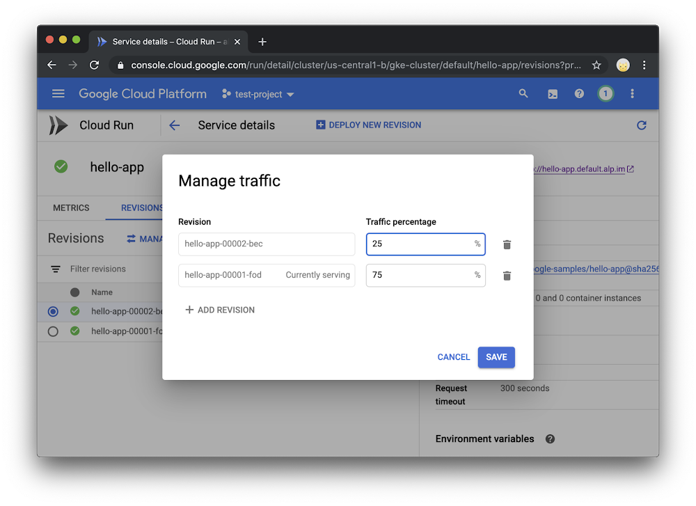
Earlier this year, we announced Cloud Run, our newest compute platform for serverless containers, which runs either on Google’s fully managed infrastructure–or on your Google Kubernetes Engine (GKE) clusters with Cloud Run for Anthos. This portability is achieved with Knative open-source APIs.With Cloud Run for Anthos, we deliver and manage everything you need to support serverless containers on your GKE clusters, for example Knative and a service mesh, and it’s now generally available. Let’s take a look at some of the new features and improvements, including better networking and autoscaling capabilities, that make it easier to deploy and operate microservices in a serverless way on your Anthos GKE clusters. (Also make sure to check out what’s new in Cloud Run fully managed.) Traffic managementCloud Run for Anthos can now route each request or RPC randomly between multiple revisions of a service with the traffic percentages you configure. You can use this feature to perform canary deployments of a newer version of your application, sending a small percentage of the traffic and validating if it is performing correctly, before gradually increasing the traffic.Similarly, these new traffic management capabilities make it possible to roll back to an older version of your application quickly. You can manage traffic to your service on the Cloud Console, as well as the gcloud command-line tool.Bringing Cloud Run to your on-prem clustersThe beta of Cloud Run for Anthos only supported GKE clusters running on Google Cloud Platform (GCP). With the general availability of Cloud Run for Anthos, you can now deploy Cloud Run to your on-premises clusters deployed on VMware.With this, you can have the same serverless developer and operator experience across both environments. You can use either gcloud or the Cloud Console to deploy to your Anthos clusters and monitor them, regardless of whether they are running on-prem, or on GCP.Support for Kubernetes Secrets and ConfigMapsYou can now mount existing Kubernetes Secret and ConfigMap resources in your cluster to Cloud Run services using the Cloud Console interface or gcloud. This lets you deploy services without crafting lengthy Kubernetes manifest files.Fine tune network and autoscaling parametersWith the new improvements in the Cloud Console and gcloud, you can now further tune the autoscaling and networking parameters of your application at per-revision level.–min-instances / –max-instances let you specify the scaling boundaries of your application. For example, setting –min-instances to greater than 0 prevents your service from scaling down to zero in case of inactivity to prevent cold starts.–timeout allows you to specify a custom request timeout for your service.–port allows you to customize and specify on which port number your containerized application is listening. This allows you to bring your apps to Cloud Run without having to modify the application server’s port number.Some of these options are currently in beta, however soon these and many other configuration options will be available to you in the command-line and the Cloud Console.Making your services more observableOut of the box, Cloud Run for Anthos integrates with Stackdriver Monitoring to expose metrics from the services you have deployed. With general availability, you can find these metrics on Stackdriver Metrics, or directly on the “Metrics” tab of the service’s Cloud Run page.These metrics include some golden signals: request latencies, error rates, CPU and memory usage, and container instance count. You can further use these metrics to drill down by revision of your application, and create alerts and SLOs using Stackdriver Monitoring.It’s also worth noting that you get the same set of metrics even if your Anthos cluster is running on-premises, for example on VMware.Smaller cluster footprintThe Istio add-on is now optional for Cloud Run for Anthos, as Cloud Run now includes select components of Istio. The full version of Istio is still a great complement to Cloud Run if you want to have cluster-wide traffic policies and use Anthos Service Mesh dashboard to have single pane of glass visibility to services in your cluster. The Istio community has recently made several improvements to Istio, including reductions in its resource footprint.Partner ecosystemWe’re working with a wide variety of ISVs in the areas of CI/CD, security and observability so that you can continue to use your favorite tools with applications running on Cloud Run for Anthos. Click here for a recent list of Cloud Run partners and integrations. Try it today!Both Cloud Run fully managed and Cloud Run for Anthos are available for you to try out for your applications today. You can try out Cloud Run on your Anthos GKE clusters by following the quickstart guide for free until May 2020. You can also use the 12-month GCP free trial to get $300 in credit and create a cluster with Cloud Run for Anthos. And if you’re already running Anthos on-premises, try this quickstart guide to deploy Cloud Run to your VMware environment.
Quelle: Google Cloud Platform

12. Dezember 2019

da Agency

Exploring container security: Performing forensics on your GKE environment

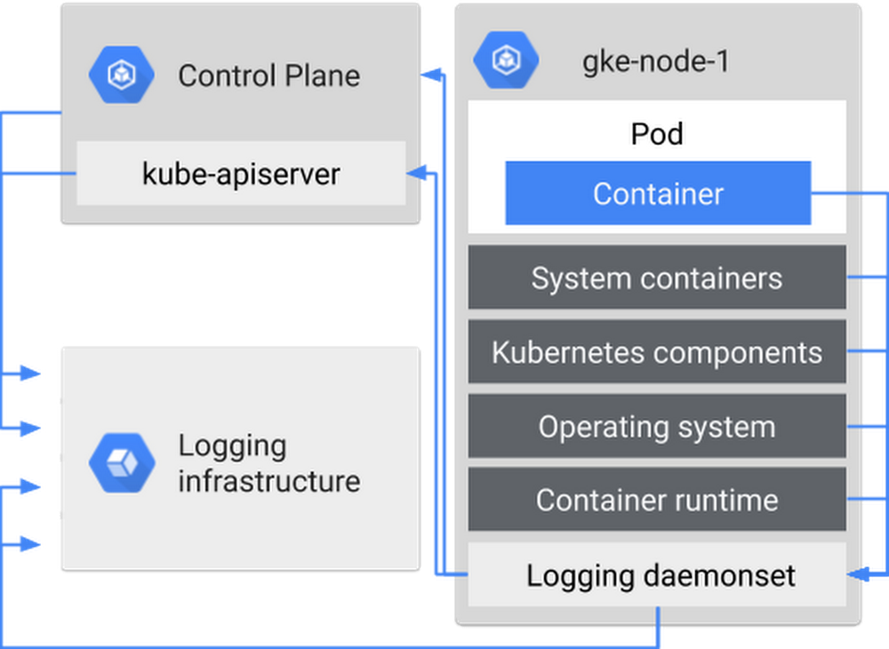
Running workloads in containers can be much easier to manage and more flexible for developers than running them in VMs, but what happens if a container gets attacked? It can be bad news. We recently published some guidance for how to collect and analyze forensic data in Google Kubernetes Engine (GKE), and how best to investigate and respond to an incident.When performing forensics on your workload, you need to perform a structured investigation, and keep a documented chain of evidence to know exactly what happened in your environment, and who was responsible for it. In that respect, performing forensics and mounting an incident response is the same for containers as it is for other environments—have an incident response plan, collect data ahead of time, and know when to call in the experts. What’s different with containers is (1) what data you can collect and how, and (2) how to react.Get planningEven before an incident occurs, make the time to put together an incident response plan. This typically includes: who to contact, what actions to take, how to start collecting information and how to communicate what’s going on, both internally and externally. Incident response plans are critical, so if panic does start to set in you’ll know what steps to follow.Other information that’s helpful to decide ahead of time, and list in your response plan, is external contacts or resources, and how your response changes based on severity of the incident. Severity levels and planned actions should be business-specific and dependent on your risks—for example, a data leak is likely more severe than an abuse of resources, and you may have different parties that need to be involved. This way, you’re not hunting around for—or debating—this information during an incident. If you don’t get the severity levels right the first time, in terms of categorization, speed of response, speed of communications, or something else, surface this in an incident post-mortem, and adjust as needed.Collect logs now, you’ll be thankful laterTo put yourself in the best possible position for responding to an incident, you want data! Artifacts such as logs, disks, and live recorded info are how you’re going to figure out what’s happening in your environment. Most of these you can get in the heat of the moment, but you need to set up logs ahead of time.There are several kinds of logs in a containerized environment that you can set up to capture: Cloud Audit Logs for GKE and Compute Engine nodes, including Kubernetes audit logs; OS specific logs; and your own application logs.There are several kinds of logs you can collect from a containerized environment.You should begin by collecting logs as soon as you deploy an app or set up a GCP project, to ensure they’re available if you need them for analysis in case of an incident. For more guidance on which logs to collect for further analysis for your containers, see our new solution Security controls and forensic analysis for GKE apps.Stay coolWhat should you do if you suspect an incident in your environment? Don’t panic! You may be tempted to terminate your pods, or restart the nodes, but try to resist the urge. Sure, that will stop the problem at hand, but it also alerts a potential attacker that you know that they’re there, depriving you of the ability to do forensics!So, what should you do? Put your incident response plan into action. Of course, what this means depends on the severity of the incident, and your certainty that you have correctly identified the issue. Your first step might be to ask your security team to further investigate the incident. The next step might be to snapshot the disk of the node that was running the container. You might then move other workloads off and quarantine the node to run additional analysis. For more ideas, check out the new documentation on mitigation options for container incidents next time you’re in such a situation (hopefully never!).To learn more about container forensics and incident response, check out our talk from KubeCon EU 2019, Container forensics: what to do when your cluster is a cluster (slides). But as always, the most important thing you can do is prevention and preparation—be sure to follow the GKE hardening guide, and set up those logs for later!
Quelle: Google Cloud Platform

12. Dezember 2019

da Agency

Performance-driven dynamic resource management in E2 VMs

Editor’s note: This is the second post in a two-post series. Click here for part 1: E2 introduction.As one of the most avid users of compute in the world, Google has invested heavily in making compute infrastructure that is cost effective, reliable and performant. The new E2 VMs are the result of innovations Google developed to run its latency-sensitive, user-facing services efficiently. In this post, we dive into the technologies that enable E2 VMs to meet rigorous performance, security, and reliability requirements while also reducing costs.In particular, the consistent performance delivered by E2 VMs is enabled by:An evolution toward large, efficient physical serversIntelligent VM placementPerformance-aware live migrationA new hypervisor CPU schedulerTogether we call these technologies dynamic resource management. Just as Google’s Search, Ads, YouTube, and Maps services benefited from earlier versions of this technology, we believe Google Cloud customers will find the value, performance, and flexibility offered by E2 VMs improves the vast majority of their workloads.Introducing dynamic resource managementBehind the scenes, Google’s hypervisor dynamically maps E2 virtual CPU and memory to physical CPU and memory on demand. This dynamic management drives cost efficiency in E2 VMs by making better use of the physical resources.Concretely, virtual CPUs (vCPUs) are implemented as threads that are scheduled to run on demand like any other thread on the host—when the vCPU has work to do, it is assigned an available physical CPU on which to run until it goes to sleep again. Similarly, virtual RAM is mapped to physical host pages via page tables that are populated when a guest-physical page is first accessed. This mapping remains fixed until the VM indicates that a guest-physical page is no longer needed.The image below shows vCPU work coming and going over the span of a single millisecond. Empty space indicates a given CPU is free to run any vCPU that needs it.A trace of 1 millisecond of CPU scheduler execution. Each row represents a CPU over time and each blue bar represents a vCPU running for a time span. Empty regions indicate the CPU is available to run the next vCPU that needs it.Notice two things: there is a lot of empty space, but few physical CPUs are continuously empty. Our goal is to better utilize this empty space by scheduling VMs to machines and scheduling vCPU threads to physical CPUs such that wait time is minimized. In most cases, we are able to do this extremely well. As a result, we can run more VMs on fewer servers, allowing us to offer E2 VMs for significantly less than other VM types.For most workloads, the majority of which are only moderately performance sensitive, E2 performance is almost indistinguishable from that of traditional VMs. Where dynamic resource management can differ in performance is in the long tail—the worst 1% or 0.1% of events. For example, a web serving application might see marginally increased response times once per 1,000 requests. For the vast majority of applications, including Google’s own latency-sensitive services, this difference is lost in the noise of other performance variations such as Java garbage collection events, I/O latencies and thread synchronization.The reason behind the difference in tail performance is statistical. Under dynamic resource management, virtual resources only consume physical resources when they are in use, enabling the host to accommodate more virtual resources than it could otherwise. However, occasionally, resource assignment needs to wait several microseconds for a physical resource to become free. This wait time can be monitored in Stackdriver and in guest programs like vmstat and top. We closely track this metric and optimize it in four ways that we detail below.1. An evolution toward large, efficient physical serversOver the past decade, core count and RAM density has steadily increased such that now our servers have far more resources than any individual E2 VM. For example, Google Cloud servers can have over 200 hardware threads available to serve vCPUs yet an E2 VM has at most 16 vCPUs. This ensures that a single VM cannot cause an unmanageable increase in load.We continually benchmark new hardware and look for platforms that are cost-effective and perform well for the widest variety of cloud workloads and services. The best ones become the “machines of the day” and we deploy them broadly. E2 VMs automatically take advantage of these continual improvements by flexibly scheduling across the zone’s available CPU platforms. As hardware upgrades land, we live-migrate E2 VMs to newer and faster hardware, allowing you to automatically take advantage of these new resources.2. Intelligent VM placementGoogle’s cluster management system, Borg, has a decade of experience scheduling billions of diverse compute tasks across diverse hardware, from TensorFlow training jobs to Search front- and back-ends. Scheduling a VM begins by understanding the resource requirements of the VM based on static creation-time characteristics.By observing the CPU, RAM, memory bandwidth, and other resource demands of VMs running on a physical server, Borg is able to predict how a newly added VM will perform on that server. It then searches across thousands of servers to find the best location to add a VM.These observations ensure that when a new VM is placed, it is compatible with its neighbors and unlikely to experience interference from those instances.3. Performance-aware live migrationAfter VMs are placed on a host, we continuously monitor VM performance and wait times so that if the resource demands of the VMs increase, we can use live migration to transparently shift E2 load to other hosts in the data center.The policy is guided by a predictive approach that gives us time to shift load, often before any wait time is encountered.VM live migration is a tried-and-true part of Compute Engine that we introduced six years ago. Over time, its performance has continually improved to the point where its impact on most workloads is negligible.4. A new hypervisor CPU schedulerIn order to meet E2 VMs performance goals, we built a custom CPU scheduler with significantly better latency guarantees and co-scheduling behavior than Linux’s default scheduler. It was purpose-built not just to improve scheduling latency, but also to handle hyperthreading vulnerabilities such as L1TF that we disclosed last year, and to eliminate much of the overhead associated with other vulnerability mitigations. The graph below shows how TCP-RR benchmark performance improves under the new scheduler.The new scheduler provides sub-microsecond average wake-up latencies and extremely fast context switching. This means that, with the exception of microsecond-sensitive workloads like high-frequency trading or gaming, the overhead of dynamic resource management is negligible for nearly all workloads.Get startedE2 VMs were designed to provide sustained performance and the lowest TCO of any VM family in Google Cloud. Together, our unique approach to fleet management, live-migration at scale, and E2’s custom CPU scheduler work behind the scenes to help you maximize your infrastructure investments and lower costs.E2 complements the other VM families we announced earlier this year—general-purpose (N2) and compute-optimized (C2) VMs. If your applications require high CPU performance for use-cases like gaming, HPC or single-threaded applications, these VM types offer great per-core performance and larger machine sizes.Delivering performant and cost-efficient compute is our bread and butter. The E2 machine types are now in beta. If you’re ready to get started, check out the E2 docs page and try them out for yourself!
Quelle: Google Cloud Platform

12. Dezember 2019

da Agency

Introducing E2, new cost-optimized general purpose VMs for Google Compute Engine

General-purpose virtual machines are the workhorses of cloud applications. Today, we’re excited to announce our E2 family of VMs for Google Compute Engine featuring dynamic resource management to deliver reliable and sustained performance, flexible configurations, and the best total cost of ownership of any of our VMs. Now in beta, E2 VMs offer similar performance to comparable N1 configurations, providing:Lower TCO: 31% savings compared to N1, offering the lowest total cost of ownership of any VM in Google Cloud.Consistent performance: Your VMs get reliable and sustained performance at a consistent low price point. Unlike comparable options from other cloud providers, E2 VMs can sustain high CPU load without artificial throttling or complicated pricing. Flexibility: You can tailor your E2 instance with up to 16 vCPUs and 128 GB of memory. At the same time, you only pay for the resources that you need with 15 new predefined configurations or the ability to use custom machine types. Since E2 VMs are based on industry-standard x86 chips from Intel and AMD, you don’t need to change your code or recompile to take advantage of this price-performance. E2 VMs are a great fit for a broad range of workloads including web servers, business-critical applications, small-to-medium sized databases and development environments. If you have workloads that run well on N1, but don’t require large instance sizes, GPUs or local SSD, consider moving them to E2. For all but the most demanding workloads, we expect E2 to deliver similar performance to N1, at a significantly lower cost. Dynamic resource managementUsing resource balancing technologies developed for Google’s own latency-critical services, E2 VMs make better use of hardware resources to drive costs down and pass the savings on to you. E2 VMs place an emphasis on performance and protect your workloads from the type of issues associated with resource-sharing thanks to our custom-built CPU scheduler and performance-aware live migration.You can learn more about how dynamic resource management works by reading the technical blog on E2 VMs.E2 machine typesAt launch, we’re offering E2 machine types as custom VM shapes or predefined configurations:We’re also introducing new shared-core instances, similar to our popular f1-micro and g1-small machine types. These are a great fit for smaller workloads like micro-services or development environments that don’t require the full vCPU.E2 VMs can be launched on-demand or as preemptible VMs. They are also eligible forcommitted use discounts, bringing additional savings up to 55% for 3 year commitments. E2 VMs are powered by Intel Xeon and AMD EPYC processors, which are selected automatically based on availability. Get startedE2 VMs are rolling out this week to eight regions: Iowa, South Carolina, Oregon, Northern Virginia, Belgium, Netherlands, Taiwan and Singapore; with more regions in the works. To learn more about E2 VMs or other GCE VM options, check out our machine types page and our pricing page.
Quelle: Google Cloud Platform

11. Dezember 2019

da Agency

Azure Sphere guardian module simplifies & secures brownfield IoT

One of the toughest IoT quandaries is figuring out how to bake IoT into existing hardware in a secure, cost-effective way. For many customers, scrapping existing hardware investments for new IoT-enabled devices (“greenfield” installations) isn’t feasible. And retrofitting mission-critical devices that are already in service with IoT (“brownfield” installations) is often deemed too risky, too complicated, and too expensive.

This is why we’re thrilled about a major advancement for Azure Sphere that opens up the brownfield opportunity, helping make IoT retrofits more secure, substantially easier, and more cost effective than ever before. The guardian module with Azure Sphere simplifies the transformation of brownfield devices into locked-down, internet-connected, data-wielding, intelligent devices that can transform business.

For an in-depth exploration of the guardian module and how it’s being used at major corporations like Starbucks, sign up for the upcoming Azure Sphere Guardian Module webinar.

The guardian module with Azure Sphere offers some key advantages

Like all Microsoft products, Azure Sphere is loaded with robust security features at every turn—from silicon to cloud. For brownfield installations, the guardian module with Azure Sphere physically plugs into existing equipment ports without the need for any hardware redesign.

Azure Sphere, rather than the device itself, talks to the cloud. The guardian module processes data and controls the device without exposing existing equipment to the potential dangers of the internet. The module shields brownfield equipment from attack by restricting the flow of data to only trusted cloud and device communication partners while also protecting module and equipment software.

Using the Azure Sphere guardian module, enterprises can enable any number of secure operations between the device and the cloud. The device can even use the Azure Sphere Security Service for certificate-based authentication, failure reporting, and software updates.

Opportunities abound for the Microsoft partner ecosystem

Given the massive scale of connectable equipment already in use in retail, industrial, and commercial settings, the new guardian module presents a lucrative opportunity for Microsoft partners. Azure Sphere can connect an enormous range of devices of all types, leading the way for a multitude of practical applications that can pay off through increased productivity, predictive maintenance, cost savings, new revenue opportunities, and more.

Fulfilling demand for such a diverse set of use cases is only possible thanks to Azure Sphere’s expanding partner ecosystem. Recent examples of this growth include our partnership with NXP to deliver a new Azure Sphere-certified chip that is an extension of their i.MX 8 high-performance applications process series and brings greater compute capabilities to support advanced workloads. As well as our collaboration with Qualcomm Technologies, Inc to deliver the first cellular-enabled Azure Sphere chip, which gives our customers the ability to securely connect anytime, anywhere.

Starbucks uses Azure Sphere guardian module to connect coffee machines

If you saw Satya Nadella’s Vision Keynote at Build 2019, you probably recall the demonstration of Starbucks’ IoT-connected coffee machines. But what you may not know is the Azure Sphere guardian module is behind the scenes, enabling Starbucks to connect these existing machines to the cloud.

As customers wait for their double-shot, no-whip mochas to brew, these IoT-enabled machines are doing more than meets the eye. They’re collecting more than a dozen data points for each precious shot, like the types of beans used, water temperature, and water quality. The solution enables Starbucks to proactively identify any issues with their machines in order to smooth their customers’ paths to caffeinated bliss.

Beyond predictive maintenance, Azure Sphere will enable Starbucks to transmit new recipes directly to machines in 30,000 stores rather than manually uploading recipes via thumb drives, saving Starbucks lots of time, money, and thumb drives. Watch this Microsoft Ignite session to see how Starbucks is tackling IoT at scale in pursuit of the perfect pour.

As an ecosystem, we have a tremendous opportunity to meet demand for brownfield installations and help our customers quickly bring their existing investments online without taking on risk and jeopardizing mission-critical equipment. The first guardian modules are available today from Avnet and AI-Link, with more expected soon.

Discover the value of adding secured connectivity to existing mission-critical equipment by registering for our upcoming Azure Sphere Guardian Modules webinar. You will experience a guided tour of the guardian module, including a deep dive into its architecture and the opportunity this open-source offering presents to our partner community. We’ll also hear from Starbucks around what they’ve learned since implementing the guardian module with Azure Sphere.
Quelle: Azure