Kategorie: Google Cloud Platform

Announcing the beta release of SparkR job types in Cloud Dataproc

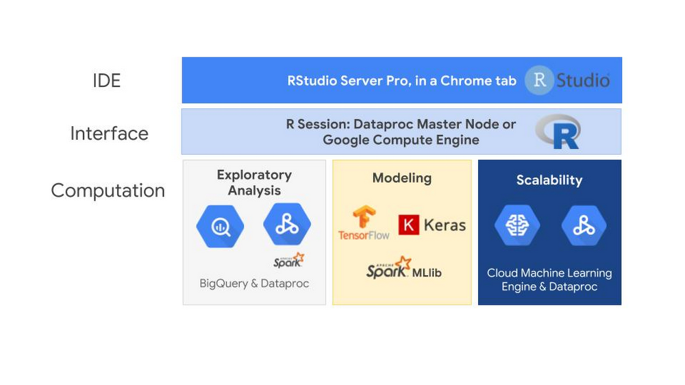
The R programming language is often used for building data analysis tools and statistical apps, and cloud computing has opened up new opportunities for those of you developing with R. Google Cloud Platform (GCP) lets you store a massive amount of data cost-effectively, then take advantage of managed compute resources only when you’re ready to scale your analysis.We’re pleased to announce the beta release of SparkR jobs on Cloud Dataproc, which is the latest chapter in building R support on GCP. SparkR is a package that provides a lightweight front end to use Apache Spark from R. This integration lets R developers use dplyr-like operations on datasets of nearly any size stored in Cloud Storage. SparkR also supports distributed machine learning using MLlib. You can use this integration to process against large Cloud Storage datasets or perform computationally intensive work.Cloud Dataproc is GCP’s fully managed cloud service for running Apache Spark and Apache Hadoop clusters in a simple and cost-efficient way. The Cloud Dataproc Jobs API makes it easy to submit SparkR jobs to a cluster without having to open firewalls to access web-based IDEs or SSH directly onto the master node. With the Jobs API, you can automate the repeatable R statistics you want to run on your datasets.Using GCP for R lets you avoid the infrastructure barriers that used to impose limits on understanding your data, such as choosing which datasets to sample because of compute or data size limits. With GCP, you can build large-scale models to analyze datasets of sizes that previously would have required huge upfront investments in high-performance computing infrastructures.What happens when you move R to the cloud?When you move R to the cloud, you’ll see the familiar RStudio interface that has served you well in prior R endeavors. While the SparkR Jobs API offers an easy way to execute SparkR code and automate tasks, most R developers will still perform the exploratory analysis using RStudio. Here’s an overview of this setup:The interface running the RStudio server could be running on either a Cloud Dataproc master node, a Google Compute Engine virtual machine or even somewhere outside of GCP entirely. One of the advantages of using GCP is that you only need to pay for the RStudio server while it is in use. You can create an RStudio server and shut it off when you’re not using it. This pay-as-you go system also applies to RStudio Pro, the commercial distribution of RStudio.The computation engines available in GCP is where using R in the cloud can really expand your statistical capabilities.The bigrquery package makes it easy to work with data stored in BigQuery by allowing you to query BigQuery tables and retrieve metadata about your projects, datasets, tables, and jobs. The SparkR package, when run on Cloud Dataproc, makes it possible to use R to analyze and structure the data stored in Cloud Storage.Once you have explored and prepared your data for modeling, you can use TensorFlow, Keras and Spark MLlib libraries. You can use the R interface to Tensorflow to work with the high-level Keras and Estimator APIs, and when you need more control, it provides full access to the core TensorFlow API. SparkR jobs on Dataproc allow you to train and score Spark MLlib models at scale. To train and host TensorFlow and Keras models at scale, you can use the R interface to Cloud Machine Learning (ML) Engine and let GCP manage the resources for you.GCP offers an end-to-end managed environment for building, training and scoring models in R. Here’s how to connect all these services in your R environment.Using RStudio: A familiar friendThe first step for most R developers is finding a way to use RStudio. While connecting to the cloud from your desktop is an option, many users prefer to have a cloud-based server version of RStudio. This helps you pick up your desktop settings from wherever you’re working, keep a backup of your work outside your personal computer, and put RStudio on the same network as your data sources. Taking advantage of Google’s high-performance network is something that can greatly improve your R performance when you move data into R’s memory space from other parts of the cloud.  If you plan to use Cloud Dataproc, you can follow this tutorialto install the open source version of RStudio server on Cloud Dataproc’s master node and access the web UI security over an SSH SOCKS tunnel. An advantage to running RStudio on Cloud Dataproc is that you can take advantage of Cloud Dataproc Autoscaling (currently in alpha). With autoscaling, you can have a minimum cluster size as you are developing your SparkR logic. Once you submit your job for large-scale processing, you don’t need to do anything different or worry about modifying your server. You simply submit your SparkR job to RStudio, and the Dataproc cluster scales to meet the needs of your job within the intervals that you set.RStudio Pro, the commercial distribution of RStudio, has a few advantages over the open source version. RStudio Server Pro provides features such as team productivity, security, centralized management, metrics, and commercial support directly from RStudio.You can even launch a production-ready deployment of RStudio Pro directly from the Google Cloud Marketplace in a matter of minutes. The instructions in the next section provide guidance on how to deploy RStudio Pro.Launch an instance of RStudio Server Pro from Cloud Launcher (optional)Cloud Marketplace contains hundreds of development stacks, solutions, and services optimized to run on GCP via one-click deployment.To launch RStudio Pro, you use the search bar at the top of the screen:Type RStudio in the Cloud Launcher search bar.Click RStudio Server Pro.Click Launch on Compute Engine.Follow the instructions. When successful, you should see a screen similar to the one below.A quick note on pricing: The page for launching an instance of RStudio Server Pro includes an estimated costs table. To the left, it also says: “Estimated costs are based on 30-day, 24 hours per day usage in Central US region. Sustained use discount is included.” However, note that most individual users use their instances intermittently and shouldn’t expect the estimated costs provided in that table. GCP has a pay-as-you-go pricing model calculated on a per-second usage basis.Submitting SparkR jobs from Cloud DataprocOnce you’ve connected R to Google Cloud, you can submit SparkR jobs using the new beta release in Cloud Dataproc. Here’s how to do that:1. Click Jobs on the left-hand side of the Dataproc user interface.2. Choose a job type of “SparkR” from the Job Type drop-down menu.3. Populate the name of an R file you want to run that is stored either on the cluster or in Cloud Storage (capital R filename required).SparkR jobs can also be used in either the gcloud betaor API. This makes it easy to automate SparkR processing steps so you can retrain models on complete datasets, pre-process data that you send to Cloud ML Engine, or generate tables for BigQuery from unstructured datasets in Cloud Storage.  When submitting a SparkR job, be sure to require the SparkR package and start the SparkR session at the top of your script.An example job output is displayed here:Connecting R to the rest of GCPAs mentioned earlier, the R community has created many packages for interacting with GCP. The following instructions can serve as a cheat sheet for quickly getting up and running with the most common packages and tools used by R developers on GCP, including SparkR.Prerequisite Python dependencies for TensorFlow stack for RStudioTensorFlow for R has two low-level Python dependencies that are difficult to install from within RStudio. If you are using RStudio Server Pro, you can SSH into the machine and run:At the time of this writing, Tensorflow is not supported directly on Cloud Dataproc due to incompatibility of operating system support.  Install additional R packagesTo generate an R session with the GCP integrations described above, run the following command in the R console:This step takes a few minutes. TensorFlow and Keras also restart your R session during installation.After installation is complete, execute the following command to confirm that the installation was successful:You can also (optionally) try out a quick check on your BigQuery by querying a public dataset:Define the connection to BigQuery from R:Then upload and collect jobs:And look at query results:Install the cloudml packageThe cloudml package is a high-level interface between R and Cloud ML Engine, Google’s platform for building massive machine learning models and bringing them to production. Cloud ML Engine provides a seamless interface for accessing cloud resources, letting you focus on model development, data processing, and inference. To get started with the cloudml package:1. Install the rstudio/cloudml package from GitHub with devtools:2. After cloudml is installed, install the Google Cloud SDK (gcloud) to interact with your Google Cloud account from within R.When you run gcloud_install, a few questions appear.3. Press ENTER to use the default values of the questions:Do you want to help improve the Google Cloud SDK (Y/N)?Do you want to continue (Y/N)?Enter a path to an rc file to update, or leave blank to use [/home/rstudio-user/.bashrc]:4. When asked which account you want to use to perform operations for this configuration, select the first account in the project (the default service account) .5. Enter the Google Cloud project ID.Using R in the cloudThis is just the start of the ways we have seen customers delving into GCP and the R ecosystem. The architecture diagram below shows an example of a full deployment of R on Google Cloud Platform for building deep learning models.To learn more about this architecture and how to get started with R on Google Cloud, check out this Next ’18 session on Getting Started with Deep Learning Models in R using Google Cloud and RStudio.For more on getting started with SparkR, check out this post or the Apache SparkR documentation.Thanks to additional contributor Michael Quinn, quantitative analyst at Google.
Quelle: Google Cloud Platform

Cloud Storage requests create data art and usage insights

The basic expectation of storage technology is that you put bytes in and you get bytes back. But storage is more insightful than you might think. At the scale of Google Cloud Platform (GCP), storage gives us a glimpse into how the world is interacting with trillions of pieces of content. When we look at storage attributes, we see the trajectory, velocity, and density of data moving around the globe. The request for a stored object gives us a piece of data about a point in time, and the origin and destination of the request at that point in time. We thought that could be thought-provoking information about a time period and a place.We on the GCP storage team wondered what the world map of those requests would look like. By exploring the planetary-level picture of our service, could we see patterns that would help us better serve our customers in the future? And, somewhat jokingly, we wondered if we could make boring old storage beautiful.So we worked with Stamen Design to take a week’s worth of our storage traffic data (aggregated and anonymized) and build a visualization that explores the interactions between users and the content stored in Google Cloud Storage. Here’s the process we used.Looking at Cloud Storage dataCloud Storage is our object storage service for storing large amounts of unstructured content. It’s a foundational element to building on GCP, and because it integrates with the majority of GCP products, it’s used for everything from audio streaming services to genomic sequencing. The service handles billions of requests a day to store or serve content from or to people and applications.  The data associated with each request made through our network tells us the direction from a country of origin to a Google Cloud region, or vice versa. This is what we call ingress (from user to Google Cloud region) and egress (from Google Cloud region to user). The associated data also tells us the size of the request in GBs and a timestamp. Since the data is anonymized, we don’t know which user is making the request, whose data is being requested or what the content is.These storage requests flow through Google’s network, which has more than 125 points of presence and thousands of miles of undersea cables.Before we get ahead of ourselves, we should clarify candidly that we were unsure this would unveil anything interesting. Given the size and simplicity of the data set, it could easily be a wash. But quick explorations using Tableau revealed a wealth of texture, with differences and similarities, and momentum for the various vectors we measured. As you can see from these initial “sketches,” movement over time was going to be key to a successful visualization, so the variable of time was our first exploration.Each image displays requests throughout the day for a country. Arrows show direction, and the size of the bubble relates to GBs in the request.Mapping time dataThe visualization below shows a snippet of the Cloud Storage data request volume over the course of a week as a series of 24-hour clocks. Each color shows data movement to a different Google Cloud region from users in the U.S., with egress flaring outwards like a coronal mass ejection, and ingress punching through towards the center of the ring—and during especially dramatic periods of ingress, even emerging out the other side.This activity generally mapped to active hours of the day for a country, with the number of requests growing toward the midday peaks. But the pattern changes day to day. We saw that spikes of ingress were far less regular than spikes of egress, and that spikes in either direction were volatile.When you think of customers who are using GCP to serve content to users, it’s easy to see why cloud elasticity is so beneficial for handling unpredictable user behavior. Behavior can be erratic. Our customers who serve global users have their own individual hourly usage patterns, and getting smarter about predicting this user behavior helps optimize for load and user experience. A pattern of consistently high requests from a country to a faraway GCP region could be better served by replicating data closer to that country, or incorporating a CDN to make the local user experience faster. The storage team is exploring how we can take insights like these and surface them to customers who would benefit.  We overlaid two countries in order to visualize their similarity in behavior, but the motion made it difficult to clearly view the differences. A radial stacked area chart simplified the data into a single, static form that still reflects the individual nature of each country and each country’s relationship with its associated GCP regions.Each radial represents 24 hours of a specific country’s Cloud Storage requests. The color represents the GCP region they transit from.These glyphs also revealed regional patterns of request volume and destination around the globe. When displayed geographically, below, you can see that continents with similar Cloud Storage traffic patterns stand out. The closer the circles are to each other in shape and color, the higher the correlation in traffic patterns.The next step was to explore whether we could visualize the expected and unexpected similarities between different sides of the world more quantitatively.Correlating time series dataBy measuring the cross-correlation of a time series, we can tell how related two time series are. If traffic in Colombia spikes, is traffic in nearby Ecuador likely to as well? What about on the other side of the world in Algeria?A cross-correlation matrix, shown below, shows this association between every pair of countries, based on Cloud Storage’s request traffic. Each country is represented on both axes of the matrix, and will meet every other at some point in the matrix. Yellow means the request pattern of the country is correlated to the country on the other axis. Blue means it’s different. The bright yellow diagonal is where a country meets itself on the other axis and the pattern is matched 100%.We can see a rich structure in this diagram. We saw correlation among continents with economic affinity, cultural cooperation, and technological collaboration across the globe. We also saw correlations between countries in proximity to each other, with users awake at the same time or using the same local GCP region.The animation above displays the cross-correlation matrix geographically, showing positive or negative correlation between each country.This made us think about how to optimize storage for both content serving and high-performance compute or analytics. Customers with very distinct global pockets of activity could architect or replicate their storage to better serve that content to users in a geographic area. If they have operations in separate areas of the globe running high-performance compute or analytics jobs, it’s a definite benefit if the job doesn’t need to traverse more distance than necessary. The closer compute is to your data, the faster you can crunch it.At this point, it was clear that correlations between countries had an interesting story to tell. Showing the characteristic pattern of each country revealed individuality in the data. Showing correlations between countries revealed connection. We laid out every country in the dataset, and drew connections between them and GCP in the circular diagram below. It’s super cool to see surges in data as they pulse between users and GCP.Pulling the pieces togetherLooking at Cloud Storage requests over time showed us a distinct pattern, the pattern gave us a way to correlate countries, and each correlation gave us an insight into connections around the globe. So we put it all together in a video that gave every country a turn in the spotlight. We included a snippet below. It jumps from country to correlated country, showing unexpected connections and prompting conversation and discussion.If you joined us at Google Cloud Next ‘18 in San Francisco, Tokyo or London, you may have seen the above as it ran in the storage and database showcase. Since it’s multiple hours long, attendees experienced a different picture or global insight each time they walked by the video.As each country is featured, you can see the textural complexity that intrigued us at the beginning of the project. Here are a few examples:How we created these Cloud Storage visualizationsThis project was mainly developed using Javascript and HTML5 Canvas. Many of the transitions and visualizations pushed the ability of Canvas to render in real time, with tens of thousands of arc segments, not to mention points, complex polygons, and text being drawn on the same frame. To deploy the final video on a Google Chromebox, we used CCapture.js, a clever library that monkey-patches Javascript’s Date function to effectively slow down time. Using some WebWorker magic, it saves each Canvas frame as an image and writes them to disk, letting us render an animation at slower than real time.If you are a Cloud Storage customer and curious about the picture your request pattern would paint, you can export the logs data for your own environment. Give the tools above a shot, or try your own. We’d love to see what you create.   Learn more about Stamen Design’s work here and Cloud Storage here.
Quelle: Google Cloud Platform

AI in depth: profiling the model training process for TensorFlow on Cloud ML Engine

If you’ve usedCloud Machine Learning (ML) Engine, you know that it can train and deploy any TensorFlow, scikit-learn, and XGBoost models at large scale in the cloud. But did you know that Cloud ML Engine also allows you to use TensorFlow’s profiling mechanisms that can help you analyze and improve your model’s performance even further?Whether you use low-level APIs such as tf.Graph and tf.Session or high-level APIs such astf.Estimator andtf.Dataset, it can sometimes be useful to understand how models perform at a lower level to tune your code for efficiency. For example, you might be interested in details about model architectures (e.g., device placement and tensor shapes) or about the performance of specific batch steps (e.g., execution time, memory consumption, or expensive operations).In this post, we show you different tools that can help you gain useful insights into your Cloud ML Engine profiling information so that you can squeeze out that extra bit of performance for your models.The examples presented in this post are based on this codelab and this notebook, which analyze a US natality dataset to predict newborns’ birth weights. While not necessary, you can follow the codelab first to familiarize yourself with the code. You can find the full code samples for this post and their prerequisites here.Basic profilingThe simplest tool at your disposal for profiling the model training process is tf.train.ProfilerHook. ProfilerHook captures profile traces for individual steps that can give you an overview of the individual TensorFlow operations (i.e., the low-level API calls associated with the nodes in your TensorFlow graph), their dependencies and how they are attributed to hardware devices (CPUs, GPUs, and TPUs). In turn, `ProfilerHook` can help you identify possible bottlenecks so you can make targeted improvements to your pipeline and choose the right Cloud ML Engine cluster configuration.If you already use TensorBoard to visualize your TensorFlow graph and store the profile traces in the same directory as the one used for your checkpoints, you will see two additional tabs named “Memory” and “Compute Time” in TensorBoard, at the bottom of the right sidebar. You will also see information about the total compute time, memory size, and tensor output shapes when clicking on a node, as described here.Capturing traces for every step over the entire training process is often impractical, because that process can become resource-intensive, significantly increase your training times, and generate volumes of information that are too large to analyze. To reduce the volume of generated information, you can lower the sampling rate by using either the save_steps or the save_secs attributes to only save profile traces respectively every N steps or N seconds. Below is an example that captures traces every 10 steps:If you want more control over which steps you’d like to profile, you can provide your own implementation of the step selection logic. For example, you can refer to LambdaProfilerHook, a custom extension of ProfilerHook that allows you to select arbitrary steps. One way to use it is to select a range of consecutive steps to profile a specific stage of the training process (in this case steps 100 to 110):ProfilerHook generates one separate trace file named timeline-[STEP_NUMBER].json in the trace-event format for each selected step. To analyze the information contained in those files, first download them locally:Then open the Chrome browser and type chrome://tracing in the URL bar. Then click the Load button and select a trace file. This loads the traces for the corresponding step into the Chrome tracing UI.In the next sections, we show you how to collect and analyze profile traces for different Cloud ML Engine scale tiers (a single machine, a distributed cluster, and a single GPU instance).Example on a single machineLet’s first take a look at some traces captured for our sample training process using the BASIC scale tier, that is, with a single worker instance with four CPUs:The above command runs the training job in 50K batch steps and generates traces every 20K steps, generating three profile trace files:After downloading and loading one of the generated files in the Chrome tracing UI, you can see the execution time and dependencies for every operation in the graph:Traces are divided in three main groups:Compute: Visualizes when each operation started and ended and in what thread it was executed. By clicking on an operation you can reveal more details about its execution times. By clicking on View options > Flow events you can reveal the operations’  dependencies.Tensors: Visualizes when each tensor was created and deleted from memory. The circles represent the exact times at which the memory snapshots were taken for each tensor. By clicking on a tensor you can get more details about its shape, memory consumption, and creation and deletion times.Allocators: Visualizes the overall memory consumption while the batch step was processed. By clicking on the barplot you can reveal the exact memory consumption values at various points in time.By inspecting the graphs, you can see that the speed or performance of your training job is mainly limited by the data input pipeline (since it’s the longest one). To implement some optimizations, you might want to check out the documentation on data input pipeline performance.Example on a distributed clusterLet’s now take a look at the same example but this time running the training job on the STANDARD_1 scale tier, i.e., one master node with four CPUs and four worker instances with eight CPUs each:The above command generates a total of 15 trace files (three for the master and three for each of the four workers). Besides the usual metrics, the workers’ trace files also contain the parameter servers’ operations. (Note: the parameter server stores and updates the model’s parameters in a distributed architecture.)If you open one of the worker’s trace files, you see that the traces divided in the same types of groups as in the first example (Compute, Tensors, and Allocators). However there are now Compute and Tensors groups for all workers (e.g., a Compute group is named /job:/worker/replica:0/task:N/device:CPU:0 Compute for an Nth worker) and for all parameter servers (e.g., a Tensors group is named /job:/ps/replica:0/task:N/device:CPU:0 Tensors for the Nth parameter server).By inspecting the graphs, you clearly see that there is some communication overhead between the nodes (that is, time spent on calls to RecvTensor):This comparison highlights the tradeoff inherent in distributed architectures: using more nodes can help the training process reach convergence quicker but also consumes more computational resources. It’s important to measure actual consumption so that you can finely adjust the number of workers you’re using, in order to reach the ideal balance between speed and cost. Capturing and visualizing traces can help you estimate your overhead, letting you more precisely select the architecture that is suited to your use case.A GPU exampleLet’s now take a look again at the same example but this time running the training job on the BASIC_GPU scale tier, that is, a single worker instance with eight CPUs and one GPU:If you open one of the generated trace files, you see that things look a bit different from our previous examples:There still is an Allocators group for the memory consumption, however multiple allocators are displayed: CPU, cpu_pool, GPU and cuda_host_buffer. You can read more about cuda_host here.Statistics about the operations run in every GPU stream (including the memcpy stream) are available in each one of the Compute groups. You can find more details about CUDA streams here or here.By inspecting the graphs, you see that the GPU utilization is quite low. This means either that GPUs are not the right fit for this model, or that the batch size must be increased significantly. You also see that the input data pipeline takes up a large share of the overall time spent for the whole step:Advanced profilingIn cases where collecting basic traces for individual steps isn’t enough, TensorFlow offers another great tool called Profiler that lets you do some advanced analysis. Profiler allows you to aggregate traces for multiple steps and calculate average values for execution times, CPU and memory consumption. It also allows you to search for the most time- or resource-expensive operations, to analyze device placement and model architecture (number of parameters, tensor shapes), and more.To use Profiler, simply instantiate a ProfileContext as shown in the following excerpt from our example code:The above code generates a single Profiler context file that contains traces for 50 consecutive steps (that is between steps #1050 and #1100). If you want more control over how Profiler traces are collected, you can customize your profiling options in the ProfilerOptionBuilder class.In the next sections, we show you two different ways to use Profiler traces: using the command line and using the standard user interface.Using Profiler with the command lineFollow these steps to use Profiler with the command line:1. Install the Bazel build tool by following the instructions for your platform. (Note: if you’ve already compiled TensorFlow from source, you should already have Bazel installed.)2. Download and compile Profiler using Bazel:3. Download the Profiler’s trace file locally:4. Start a new Profiler session:Now let’s take a look at a few examples of what you can do in Profiler by passing different options to the command line tool:1. Display the python methods invocation tree:The above command displays average statistics for the 50 profiled steps. You can also specify the exact steps that you are interested in by using the `regExes` filters.2. Expose the operations that consume the most memory:3. Display the tensor shapes and the number of parameters for all calls made to tf.trainabale_variables() in the profiled training steps:Lastly, you can also experiment with the advise command to automatically profile your model and easily find the most expensive operations, the accelerators’ utilization, and more.You can also visualize a timeline for a specific step to inspect with chrome://tracing as we’ve discussed above (read more about how to do this), or generate your own timelines for a few steps. First,  generate a binary profile (taking into account your desired conditions) and then generate a visualization with pprof (if you’ve installed it):tfprof> code -select accelerator_micros -max_depth 100000 -output pprof:outfile=PATH_TO_YOUR_FILE  -trim_name_regexes .*apply_op.*And now execute this command from your terminal to generate a png file:Using the Profiler UIThere’s also a user interface tool called profiler-ui to analyze your Profiler trace files. To use profiler-ui, first follow the installation instructions, then start the tool:This tool has the same capabilities as the command line interface but it is generally easier to use and can help you visually identify bottlenecks in the flow of operations.ConclusionWe hope you find these techniques useful when training models, to better understand the performance and behavior of your training process. If you’re interested in learning more, check out some of our documentation below:Cloud ML Engine documentationTensorFlow guide to collecting runtime statisticsTensorFlow Profiler documentationTensorFlow CLI profiling tool optionsTraceEvent format for TensorFlowChromium Trace event profiling toolTensorflow Model Benchmark tool for inference profiling
Quelle: Google Cloud Platform

New for Persistent Disk and Compute Engine: Control the storage location of your disk snapshots

Google Compute Engine lets you create a snapshot for a persistent disk in order to provide  point-in-time data protection for that disk. We’re pleased to let you know that you can now specify the storage location of your snapshots down to the regional level with the new snapshot feature in beta. You can specify snapshot locations at the regional or multi-regional level, which map to the Google Cloud Storage regional and multi-regional locations, for example, “us-central1” or “us”.The ability to select a specific storage location for your snapshots provides you with a greater level of control over where your snapshots are stored. This is particularly helpful to meet data residency and business continuity requirements. Visit the pricing page to understand the cost of snapshot storage and network transit (Pricing is subject to change once the snapshot location feature is Generally Available (GA)).Choosing your snapshot location with Compute EngineTo get started with this new feature, use the newly-added -storageLocation property in the disks.createSnapshot() beta API, or use the gcloud command example below:You can also control the storage location of snapshots when you create a new snapshot in the Developer Console, as pictured below.Specifying a regional location can be especially helpful when you’re trying to meet regulatory and compliance requirements, like storing patient health records or customer financial data in a particular location. By choosing a multi-regional storage location, you benefit from data redundancy across multiple data centers that are separated by at least 100 miles. This provides the highest availability for your data, even in the event of large-scale disruptions.Whether you choose a regional or multi-regional location, you can still access your snapshot as a globally addressable Compute Engine resource. This makes it easy to build cross-region systems, since you can reference your snapshots from any region.Get started by trying out this new snapshot feature in the Developer Console, through gcloud or using the API. You can also check out the documentation to learn more details.
Quelle: Google Cloud Platform

Cloud Identity for Customers and Partners (CICP) is now in beta and ready to use

In October at Next ’18 London, we announced Cloud Identity for Customers and Partners (CICP) to help you add Google-grade identity and access management (IAM) functionality to your apps, protect user accounts, and scale with confidence—even if those users are customers, partners, and vendors who might be outside of your organization. CICP is now available in public beta.Adding Google-grade authentication to your appsAll users expect simple and secure sign-up, sign-in, and self-service experiences from all their devices. While you could build an IAM system for your apps, it can be hard and expensive. Just think about the complexity of building and maintaining an IAM system that stays up-to-date with evolving authentication requirements, keeping user accounts secure in the face of threats that increase in occurrence and sophistication, and scaling the system reliably when the demand for your app grows.Cloud Identity for Customers and Partners (CICP) is a customer identity and access management (CIAM) platform that addresses these issues and lets you focus on building your apps by delivering essential IAM and user security capabilities such as:Google-grade authentication. Based on Firebase and Google’s identity platforms, CICP provides a drop-in, customizable authentication service that manages the UI flows for user sign-up and sign-in. CICP also supports multiple authentication methods (anonymous, email/password, phone, social, SAML, OIDC, and more), client SDKs (web, iOS, and Android), and server SDKs (Node.js, Java, Python, and more).Advanced user security. CICP is integrated with Google’s intelligence and threat signals to help detect compromised user accounts. We are also working to enable two-factor authentication (2FA), when CICP becomes generally available, to help protect users from phishing attacks and account takeovers.Planet-scale infrastructure. Built on Google Cloud’s highly secure, performant and scalable infrastructure, CICP is designed to satisfy the needs of even the most demanding applications. When CICP reaches general availability, it will also include an enterprise-grade availability SLA and technical support to give you peace of mind about this foundational component of your app environment.Getting startedCICP is now being gradually rolled out. To get started, enable customer identity in GCP Marketplace and check out the quickstart for how-to guides.
Quelle: Google Cloud Platform

Taking a practical approach to BigQuery cost monitoring

Google BigQuery is a serverless enterprise data warehouse tool that’s designed for scalability. We built BigQuery to be highly scalable and let you focus on data analysis without having to take care of the underlying infrastructure. We know BigQuery users like its capability to query petabyte-scale datasets without the need to provision anything. You just upload the data and start playing with it.BigQuery comes with two different pricing models:The on-demand model, where users are charged for the amount of TB of data to be processed by their queries;The flat model, suitable for customers who want to pay a monthly fixed cost to be able to execute unlimited queries, regardless of the amount of processed data.When our users choose the on-demand option, we often get one question: How can I monitor the spending of my users? Here, we’ll show you how to implement a fully serverless solution for near–real-time cost monitoring using readily available log data.To achieve this, we’ll build a Data Studio dashboard (easily integrated into BigQuery) to report the daily BigQuery spending split by users at a particular organization. In this example, the daily cost to the organization was $95.95, with three users contributing to that total.Daily BigQuery usage cost, split by usersHere’s how to build your own dashboard to monitor BigQuery usage costs.Collect the necessary log dataAll the information you need to build the cost monitoring dashboard is available through the Cloud Audit Log service in Google Cloud Platform (GCP), which keeps track of all the events generated by BigQuery, such as the creation of a table, a data insertion or a query execution. The system will log all the operations, and you can then see the entries in GCP’s Stackdriver logging and monitoring tool. Here’s an example of a list of BigQuery events shown in Stackdriver:To build a cost monitoring dashboard, you’ll need the information tied to the events tagged “query_job_completed.” If you select one of those events and expand it, you’ll see several details about the query that was executed, like the SQL code, the job ID and, most important, the user who executed the query and the amount of data that was processed. With that information, you can compute the total cost of the query using a simple multiplication equation: cost per TB processed * numbers of TB processed.Move log data into BigQuery tablesOnce you’ve identified your data, the fastest way to generate a dashboard using Data Studio is to input all the information into (guess where?) BigQuery. To do that, use the sink feature of Stackdriver to activate a streaming pipeline to ingest logs into BigQuery, in close to real time. You’ll need to define the subset of information that’s needed (in this case, all the BigQuery “query_job_completed” events) and create a sink that has BigQuery as the target. Data will automatically flow into daily BigQuery tables as soon as it is collected by the Cloud Audit Log service.Note that you can export logs of all the projects within your organization by using the aggregated exports feature. However, you’ll need to have appropriate IAM access.Create a targeted viewOnce the raw data is available in BigQuery, create a dedicated view that contains only the information needed to generate the dashboard:The name of the user who executed the queryThe cost of the queryOnce you have that information, use the following query to generate a BigQuery view that computes daily user spending based on the raw data collected from Stackdriver.Note that the above SQL code will automatically select the data for the current day. Also note that this query uses the current on-demand pricing for the EU and U.S. to compute the total cost of a query; pricing could vary for other regions. Returned data is related to list pricing and does not reflect any eventual discounts or credits that can be applied at the billing account level. For details about overall GCP billing, you can export the data to BigQuery using the native export function.Build a Data Studio dashboardNow that you’ve defined your BigQuery view with the necessary data, it is simple to use Data Studio to create a dashboard that sums up all the costs and groups them by user. You’ll end up with a dashboard that can be shared with anyone who wants to monitor daily BigQuery on-demand spending.That’s one small subset of the information BigQuery makes available. We encourage you to dig into your BigQuery data to find other elements that could be interesting for you and your business (a small hint: try cached queries ).
Quelle: Google Cloud Platform

Enterprise IT can move up or out (or both)

Much of what we do at Google Cloud’s Office of the CTO, or OCTO, is to help customers plan and execute their cloud migrations, which are often part of a larger transformation effort. Most CIOs see a cloud migration as an essential, but still somewhat daunting task. We have distilled the conversations we’ve had with CIOs, CTOs, and their technical staff into several frameworks that can help cut through the hype and the technical complexity to help devise the strategy that empowers both the business and IT. We called one such framework “up or out.” And we don’t mean some consulting firm’s hard-nosed career philosophy.The trouble with on-premises ITWhile on-premises IT infrastructure has gotten much better over the past couple of decades, e.g. through virtualization or software-defined networks, enterprise IT remains relatively inflexible, labor-intensive and slow to provision or configure infrastructure. In a slow-moving environment, this kind of setup was adequate because business demand could be predicted well ahead of time and sudden workload spikes were rare. However, digital disruptors and cost pressures force businesses and IT alike to move faster, placing significant strain on existing technologies and processes.  Migrating to the cloud: up, out, or both?A cloud-based IT operating model has been shown to offer significant advantages in terms of rapid deployment, elastic scalability, resilient operations, and security. However, large enterprises can’t simply wake up one day with all their applications running in the cloud. Thus, every enterprise’s move to the cloud is at least initially a hybrid cloud scenario, where some workloads remain on-premises and other workloads run in the cloud.Additionally, many enterprises rely on geographically distributed compute capacity and data storage that can’t be simply centralized into a single cloud data center. For example, most retail or manufacturing businesses have a significant IT footprint in branches or plants due to latency considerations or to assure continued operations in case of a network failure. Hence, when planning an enterprise cloud migration, you can’t simply move all your infrastructure overnight, but must take a more pragmatic approach that differentiates between workloads and data more carefully.One model that we found can help enterprises chart their cloud adoption journey delineates cloud migration along two axes—up and out.Up the stackOne choice you can make is to move your applications up the stack. As an initial step, you can transition from running monolithic applications on dedicated servers to a Platform-as-a-Service model that deploys applications and services using containers, managed by Kubernetes or Google Kubernetes Engine (GKE). So-called serverless deployment, for example with Cloud Functions, takes it one step further with individual application functions that hide all the infrastructure underneath.Moving up the stack has several advantages:Application deployment becomes automated, making it easy to add or subtract capacity as needed.Operations also become more resilient because new instances can be rapidly deployed in case of failure, allowing Platform-as-a-Service or serverless platforms to withstand a server failure without visible customer impact.Thanks to smaller deployable units, hardware can be more efficiently utilized, thus reducing run costs.Lastly, applications become more portable when they are better isolated from infrastructure details, as their containers may be deployed on a variety of infrastructures. This paves the way for a hybrid cloud scenario that provides a consistent service execution environment across the entire estate, including cloud vendors, on-prem data centers, branch locations, and remote devices.On the flipside, moving up the stack requires you to fundamentally change the way in which you build applications and operate the infrastructure that supports them.Out into the cloudThe second option is to lift, shift, and replatform existing applications largely unchanged out into the cloud, for example by moving virtual machines to Compute Engine or by replacing on-premise data archiving with cold-line Cloud Storage. Shifting workloads in the cloud can be simplified and even automated, for example by using tools like Velostrata.Even though the applications don’t change, moving them from an existing on-premises data center to the cloud and shifting the operational model to one that’s more automated also has several advantages:Better economies of scale allow for more cost-efficient operations.Automated patching discipline improves security because it assures that no software with known vulnerabilities is run.Increased transparency enables more efficient IT asset management, for example by rightsizing servers or detecting and retiring unused IT assets.Moving out into the cloud transforms how an enterprise operates and acquires IT infrastructure from an asset-based model to usage-based model. It’s not a black-or-white scenario, however. Similar to transforming application architectures to move ‘up’ the stack towards cloud-native systems and services architecture, moving ‘out’ to cloud can be seen as a progressive transformation toward cloud-centric operations.Lifting existing applications and replatforming them onto cloud infrastructure minimizes initial effort, avoiding the costs of redevelopment, and allowing an enterprise to transform its infrastructure acquisition and scaling processes while minimizing impact to existing operations models.Adjusting operations models to increase the use of automation and cloud-native tooling accelerates the overall transformation and maximizes the value from abstracted infrastructure services.Finally, decomposing application elements to take advantage of managed cloud services, such as migrating off of self-managed My SQL databases onto  provider-managed Database-as-a-Service, requires some additional effort but lays the foundation for moving beyond seeing cloud as yet another infrastructure provider.Not only is combining up and out allowed, it’s encouraged. We think of it as a cloud-native hybrid model, where applications are deployed as containers or functions and can be easily shifted from on-premises to the cloud as needed, all while maintaining a consistent deployment, run-time, and management framework.Plotting a migration pathThere isn’t a single path to the cloud—not for individual enterprises and not even for individual applications. Sadly, inspired by the hope for simplicity, enterprises often assume that all workload migrations will follow a common trajectory. Rather, we recommend that you use a framework that encourages flexibility. The up or out framework can help an IT organization and its leadership characterize how they can best benefit from migrating their services or workloads. The framework acts as a general pattern that highlights the continuum of approaches to explore. Not all components of a single workload will follow the same path, nor should they.Consider a few questions to ask:Which elements of an application or service would benefit most from an event-driven, serverless approach?Which elements of a service require rapid code releases or the ability to validate new features using A/B testing (meaning that a new version of the software is made available to a percentage of users)?Which elements change infrequently, but would benefit from automated scaling and deployment?With the answers to these questions, you can begin to decompose workloads (if amenable) and map them against the up or out framework, thus presenting the organization with a pragmatic migration approach that maximizes value.Applying the modelWhen a major retailer started migrating to GCP, the up or out model helped them decide which parts of their IT estate should follow which path. The retailer’s user-facing front end required frequent feature releases to remain ahead in a competitive retail market to gauge adoption and the user value of new features. A/B testing was needed to meet these needs, while an automated CI/CD pipeline deployed cloud-native applications to Google Kubernetes Engine (GKE), moving these applications both up the stack and out into the cloud.The retailer’s mid-tier application processing could also benefit from refactoring and re-architecting over time, but more immediate value could be generated by shifting to an automated scale-out model and gaining operational efficiencies in the cloud. These applications were moved to Google Compute Engine.The retailer’s back-end catalog systems change quite rarely and were hosted on well-understood and easily maintained systems. To focus their initial energy, they decided to keep these systems in place until they can replace them completely in the future.Taking this approach allowed the retailer to minimize the time and effort required to accomplish their primary goal—rapid iteration of a customer experience that was becoming stale. They also gained operational and capital efficiencies and set themselves in a good position to migrate their catalog data to the cloud when the time and price were right for them.ConclusionWhen planning a cloud migration, plotting a path for individual workloads and architectural elements on the up or out framework helps IT decision makers focus on the benefits achieved by re-platforming, re-architecting, or a combination of the two.  It also communicates migration paths over time in an approachable manner that can be shared with a wide audience in both business and IT. It’s typical and in fact desired that different components take unique paths. Whatever the best path may be, Google Cloud Platform includes the needed products and migration tools, ranging from lift-and-shift to Compute Engine, porting applications to GKE on premises or in the cloud, or deploying cloud-native services to Cloud Functions.Next stepsSimple but evocative frameworks like up or out can help IT decision makers navigate the inevitable complexity of a cloud migration. Like any good model, simplicity is a feature, not a bug, as it helps keep the focus on the desired outcome and is easily communicated to a variety of audiences.Plotting the adoption paths for different parts of your IT estate is an important first step. In subsequent articles we’ll dive in a bit deeper and explore some of the technology and architecture transformations that each of these paths implies.
Quelle: Google Cloud Platform