Microsoft has validated the Lenovo ThinkSystem SE350 edge server for Azure Stack HCI

Do you need rugged, compact-sized hyperconverged infrastructure (HCI) enabled servers to run your branch office and edge workloads? Do you want to modernize your applications and IoT functions with container technology? Do you want to leverage Azure's hybrid services such as backup, disaster recovery, update managment, monitoring, and security compliance?  

Microsoft and Lenovo have teamed up to validate the Lenovo ThinkSystem SE350 for Microsoft's Azure Stack HCI program. The ThinkSystem SE350 was designed and built with the unique requirements of edge servers in mind. It is versatile enough to stretch the limitations of server locations, providing a variety of connectivity and security options and can be easily managed with Lenovo XClarity Controller. The ThinkSystem SE350 solution has a focus on smart connectivity, business security, and manageability for the harsh environment. To see all Lenovo servers validated for Azure Stack HCI, see the Azure Stack HCI catalog to learn more.

Lenovo ThinkSystem SE350:

The ThinkSystem SE350 is the latest workhorse for the edge. Designed and built with the unique requirements for edge servers in mind, it is versatile enough to stretch the limitations of server locations, providing a variety of connectivity and security options and is easily managed with Lenovo XClarity Controller. The ThinkSystem SE350 is a rugged compact-sized edge solution with a focus on smart connectivity, business security, and manageability for the harsh environment.

The ThinkSystem SE350 is an Intel® Xeon® D processor-based server, with a 1U height, half-width and short depth case that can go anywhere. Mount it on a wall, stack it on a shelf, or install it in a rack. This rugged edge server can handle anything from 0-55°C as well as full performance in high dust and vibration environments.

Information availability is another challenging issue for users at the edge, who require insight into their operations at all times to ensure they are making the right decisions. The ThinkSystem SE350 is designed to provide several connectivity options with wired and secure wireless Wi-Fi and LTE connection ability. This purpose-built compact server is reliable for a wide variety of edge and IoT workloads.

Microsoft Azure Stack HCI:

Azure Stack HCI solutions bring together highly virtualized compute, storage, and networking on industry-standard x86 servers and components. Combining resources in the same cluster makes it easier for you to deploy, manage, and scale. Manage with your choice of command-line automation or Windows Admin Center.

Achieve industry-leading virtual machine (VM) performance for your server applications with Hyper-V, the foundational hypervisor technology of the Microsoft cloud, and Storage Spaces Direct technology with built-in support for non-volatile memory express (NVMe), persistent memory, and remote direct memory access (RDMA) networking.

Help keep apps and data secure with shielded virtual machines, network micro-segmentation, and native encryption.

You can take advantage of cloud and on-premises working together with a hyper-converged infrastructure platform in the public cloud. Your team can start building cloud skills with built-in integration to Azure infrastructure management services:

Azure Site Recovery for high availability and disaster recovery as a service (DRaaS).

Azure Monitor, a centralized hub to track what’s happening across your applications, network, and infrastructure, with advanced analytics powered by artificial intelligence.

Cloud Witness, to use Azure as the lightweight tie-breaker for cluster quorum.

Azure Backup for offsite data protection and to protect against ransomware.

Azure Update Management for update assessment and update deployments for Windows Virtual Machines running in Azure and on-premises.

Azure Network Adapter to connect resources on-premises with your VMs in Azure via a point-to-site VPN.

Sync your file server with the cloud, using Azure File Sync.

Azure Arc for Servers to manage role-based access control, governance, and compliance policy from Azure Portal.

By deploying the Microsoft + Lenovo HCI solution, you can quickly solve your branch office and edge needs with high performance and resiliency while protecting your business assets by enabling the Azure hybrid services built into the Azure Stack HCI Branch office and edge solution.  
Quelle: Azure

Managing the TICK Stack with Docker App

Photo by Sergio Souza on Unsplash
Docker Application eases the packaging and the distribution of a Docker Compose application. The TICK stack – Telegraf, InfluxDB, Chronograf, and Kapacitor – is a good candidate to illustrate how this actually works. In this blog, I’ll show you how to deploy the TICK stack as a Docker App.
About the TICK Stack
This application stack is mainly used to handle time-series data. That makes it a great choice for IoT projects, where devices send data (temperature, weather indicators, water level, etc.) on a regular basis.
Its name comes from its components:
– Telegraf
– InfluxDB
– Chronograf
– Kapacitor
The schema below illustrates the overall architecture, and outlines the role of each component.

Data are sent to Telegraph and stored in an InfluxDB database. Chronograf can query the database through a web interface. Kapacitor can process, monitor, and raise alerts based on the data.
Defining the Application in a Compose File
The tick.yml file below defines the four components of the stack and the way they communicate with each other:
version: ‘3.7’
services:
  telegraf:
    image: telegraf
    configs:
    – source: telegraf-conf
      target: /etc/telegraf/telegraf.conf
    ports:
    – 8186:8186
  influxdb:
    image: influxdb
  chronograf:
    image: chronograf
    ports:
    – 8888:8888
    command: [“chronograf”, “–influxdb-url=http://influxdb:8086″]
  kapacitor:
    image: kapacitor
    environment:
    – KAPACITOR_INFLUXDB_0_URLS_0=http://influxdb:8086
configs:
  telegraf-conf:
    file: ./telegraf.conf
Telegraf’s configuration is provided through a Docker Config object, created out of the following telegraf.conf file:
[agent]
  interval = “5s”
  round_interval = true
  metric_batch_size = 1000
  metric_buffer_limit = 10000
  collection_jitter = “0s”
  flush_interval = “5s”
  flush_jitter = “0s”
  precision = “”
  debug = false
  quiet = false
  logfile = “”
  hostname = “$HOSTNAME”
  omit_hostname = false
[[outputs.influxdb]]
  urls = [“http://influxdb:8086″]
  database = “test”
  username = “”
  password = “”
  retention_policy = “”
  write_consistency = “any”
  timeout = “5s”
[[inputs.http_listener]]
  service_address = “:8186″
[cpu]
  # Whether to report per-cpu stats or not
  percpu = true
  # Whether to report total system cpu stats or not
  totalcpu = true
This configuration:

Defines an agent that gathers host CPU metrics on a regular basis.
Defines an additional input method allowing Telegraf to receive data over HTTP.
Specifies the name of the database the data collected/received will be stored.

Deploying the application from Docker Desktop
Now we will deploy the application using Swarm first, and then using Kubernetes to illustrate some of the differences.
Using Swarm to Deploy the TICK Stack
First we setup a local Swarm using the following command:
$ docker swarm init
Then we deploy the TICK stack as a Docker Stack:
$ docker stack deploy tick -c tick.yaml
Creating network tick_default
Creating config tick_telegraf-conf
Creating service tick_telegraf
Creating service tick_influxdb
Creating service tick_chronograf
Creating service tick_kapacitor
This creates:

A network for communication between the application containers 
A Config object containing the Telegraf configuration we defined in telegraf.conf
The 4 services composing the TICK stack

It only takes a couple of seconds before the application is up and running. Now we can verify the status of each service.
$ docker service ls
ID                  NAME MODE                REPLICAS IMAGE PORTS
74zkf54ruztg        tick_chronograf replicated          1/1 chronograf:latest *:8888->8888/tcp
y97hcx3yyjx6        tick_influxdb replicated          1/1 influxdb:latest
fm4uckqlvhvt        tick_kapacitor replicated          1/1 kapacitor:latest
12zl0sa678xh        tick_telegraf replicated          1/1 telegraf:latest *:8186->8186/tcp
Only Telegraf and Chronograf are exposed to the outside world:

Telegraf is used to ingest data through port 8186
Chronograf is used to visualize the data and is available through a web interface on local port 8888

To query data from the Chronograf interface, we first need to send some data to Telegraf.
Sending Test data
First we will use the lucj/genx Docker image to generate data following a cosine distribution (a couple of other simple distributions are available).
$ docker run lucj/genx
Usage of /genx:
 -duration string
      duration of the generation (default “1d”)
 -first float
      first value for linear type
 -last float
      last value for linear type (default 1)
 -max float
       max value for cos type (default 25)
 -min float
       min value for cos type (default 10)
 -period string
       period for cos type (default “1d”)
 -step string
       step / sampling period (default “1h”)
 -type string
       type of curve (default “cos”)
We will generate three days of data, with a one day period, min/max values of 10/25 and a sampling step of one hour; that will be enough for our tests.
$ docker run lucj/genx:0.1 -type cos -duration 3d -min 10 -max 25 -step 1h > /tmp/data
We then send the data to the Telegraf HTTP endpoint with the following commands:
PORT=8186
endpoint=”http://localhost:$PORT/write”
cat /tmp/data | while read line; do
  ts=”$(echo $line | cut -d’ ‘ -f1)000000000″
  value=$(echo $line | cut -d’ ‘ -f2)
  curl -i -XPOST $endpoint –data-binary “temp value=${value} ${ts}”
done
Next, from the Explore tab in the Chronograf web interface we can visualize the data using the following query:
select “value” from “test”.”autogen”.”temp”
We will see a neat cosine distribution:

With just a couple of commands, we have deployed the TICK stack on a Swarm cluster, sent time series data and visualized it.
Finally, we remove the stack:
$ docker stack rm tick
Removing service tick_chronograf
Removing service tick_influxdb
Removing service tick_kapacitor
Removing service tick_telegraf
Removing config tick_telegraf-conf
Removing network tick_default
We have shown how to deploy the application stack with Docker Swarm. Now we will deploy it with Kubernetes.
Using Kubernetes to Deploy the TICK Stack
From Docker Desktop, deploying the same application on a Kubernetes cluster is also a simple process.
Activate Kubernetes from Docker Desktop
First, activate Kubernetes from the Docker Desktop settings:

A local Kubernetes cluster starts quickly and is accessible right from our local environment.

When the Kubernetes cluster is created, a configuration file (also known as kubeconfig) is created locally (usually in ~/.kube/config), or used to enrich this file if it already exists. This configuration file contains all the information needed to communicate with the API Server securely:

The cluster’s CA
The API Server endpoint
The default user’s certificate and private key

Creating a new Docker context
Docker 19.03 introduced the context object. It allows you to quickly switch the CLI configuration to connect with different clusters. A single context exists by default as shown below:
$ docker context list
NAME                DESCRIPTION                       DOCKER ENDPOINT KUBERNETES ENDPOINT                           ORCHESTRATOR
default *           Current DOCKER_HOST based configuration   unix:///var/run/docker.sock https://kubernetes.docker.internal:6443 (default)   swarm
Note: as we can see from the ORCHESTRATOR column, this context can only be used to deploy workload on the local Swarm.
We will now create a new Docker context dedicated to run Kubernetes workloads. This can be done with the following command:
$ docker context create k8s-demo
  –default-stack-orchestrator=kubernetes
  –kubernetes config-file=$HOME/.kube/config
  –description “Local k8s from Docker Desktop”
  –docker host=unix:///var/run/docker.sock
Next, we verify that both contexts are now available:
$ docker context list
NAME                DESCRIPTION                       DOCKER ENDPOINT KUBERNETES ENDPOINT                           ORCHESTRATOR
default *           Current DOCKER_HOST based configuration   unix:///var/run/docker.sock https://kubernetes.docker.internal:6443 (default)   swarm
k8s-demo            Local k8s from Docker Desktop             unix:///var/run/docker.sock https://kubernetes.docker.internal:6443 (default)   kubernetes
Note: we could use a single context where both orchestrators are defined. In that case, the deployment would be done on Swarm and Kubernetes at the same time.
Next, we switch on the k8s-demo context:
$ docker context use k8s-demo
k8s-demo
Current context is now “k8s-demo”
Then we deploy the application in the same way we did before, but this time it will run on Kubernetes instead of Swarm.
$ docker stack deploy tick -c tick.yaml
Waiting for the stack to be stable and running…
chronograf: Ready [pod status: 1/1 ready, 0/1 pending, 0/1 failed]
influxdb: Ready [pod status: 1/1 ready, 0/1 pending, 0/1 failed]
kapacitor: Ready [pod status: 1/1 ready, 0/1 pending, 0/1 failed]
telegraf: Ready [pod status: 1/1 ready, 0/1 pending, 0/1 failed]

Stack tick is stable and running
Using the usual kubectl binary, we can verify all the Kubernetes resources have been created:
$ kubectl get deploy,po,svc
NAME                               READY UP-TO-DATE AVAILABLE AGE
deployment.extensions/chronograf   1/1 1 1 2m50s
deployment.extensions/influxdb     1/1 1 1 2m50s
deployment.extensions/kapacitor    1/1 1 1 2m49s
deployment.extensions/telegraf     1/1 1 1 2m49s

NAME                             READY STATUS RESTARTS AGE
pod/chronograf-c55797884-mp8gc   1/1 Running 0 2m50s
pod/influxdb-67c574845d-z6846    1/1 Running 0 2m50s
pod/kapacitor-57f6787666-t8j6l   1/1 Running 0 2m49s
pod/telegraf-6b8648884c-lq9t5    1/1 Running 0 2m49s

NAME                           TYPE CLUSTER-IP EXTERNAL-IP   PORT(S) AGE
service/chronograf             ClusterIP None <none>        55555/TCP 2m49s
service/chronograf-published   LoadBalancer 10.105.63.34 <pending>     8888:32163/TCP 2m49s
service/influxdb               ClusterIP None <none>        55555/TCP 2m49s
service/kapacitor              ClusterIP None <none>        55555/TCP 2m49s
service/kubernetes             ClusterIP 10.96.0.1 <none>        443/TCP 30h
service/telegraf               ClusterIP None <none>        55555/TCP 2m49s
service/telegraf-published     LoadBalancer 10.107.223.80 <pending>     8186:32460/TCP 2m49s
We can generate some dummy data and visualize them using Chronograf following the same process we did above for Swarm (I only show the result here as the process is the same):

Finally we remove the stack:
$ docker stack rm tick
Removing stack: tick
Note: we used the same command to remove the stack from Kubernetes or Swarm, but notice the output is not the same as each orchestrator handles different  resources / objects.
Defining the TICK stack as a DockerApp
We followed simple steps to deploy the application using both Swarm and Kubernetes. Now we’ll define it as a Docker Application to make it more portable, and see how it eases the deployment process. 
Docker App is shipped with Docker 19.03+ and can be used once the experimental flag is enabled for the CLI. This can be done in several ways:

modifying the config.json file (usually in the $HOME/.docker folder)

{
“experimental”: “enabled”
}

setting the DOCKER_CLI_EXPERIMENTAL environment variable

export DOCKER_CLI_EXPERIMENTAL=enabled
Once this is done, we can check that Docker App is enabled:
$ docker app version
Version: v0.8.0
Git commit: 7eea32b7
Built: Tue Jun 11 20:53:26 2019
OS/Arch: darwin/amd64
Experimental: off
Renderers: none
Invocation Base Image: docker/cnab-app-base:v0.8.0
Note: version 0.8 is currently the last version
Note: the Docker App command is experimental, which means that the feature is subject to change before being ready for production. The user experience will be updated in the next release.
Available commands in Docker App
Several commands are available to manage the lifecycle of a Docker Application, as we can see below. We will illustrate some of them later in this article.
$ docker app

Usage: docker app COMMAND

A tool to build and manage Docker Applications.

Commands:
bundle Create a CNAB invocation image and `bundle.json` for the application
completion Generates completion scripts for the specified shell (bash or zsh)
init Initialize Docker Application definition
inspect Shows metadata, parameters and a summary of the Compose file for a given application
install Install an application
list List the installations and their last known installation result
merge Merge a directory format Docker Application definition into a single file
pull Pull an application package from a registry
push Push an application package to a registry
render Render the Compose file for an Application Package
split Split a single-file Docker Application definition into the directory format
status Get the installation status of an application
uninstall Uninstall an application
upgrade Upgrade an installed application
validate Checks the rendered application is syntactically correct
version Print version information

Run ‘docker app COMMAND –help’ for more information on a command.

Creating a Docker Application Package for the TICK stack
We start with the folder which contains the Docker Compose file describing the application (tick.yml) and the Telegraf configuration file (telegraf.conf):
$ tree .
.
├── telegraf.conf
└── tick.yml
Next we create the Docker Application, named tick:
$ docker app init tick –compose-file tick.yml –description “tick stack”
Created “tick.dockerapp”
This creates the folder tick.dockerapp, and three additional files:
$ tree .
.
├── telegraf.conf
├── tick.dockerapp
│ ├── docker-compose.yml
│ ├── metadata.yml
│ └── parameters.yml
└── tick.yml

1 directory, 5 files

– docker-compose.yml is the copy of the tick.yml file- metadata.yml defines metadata and additional parameters
$ cat tick.dockerapp/metadata.yml
# Version of the application
version: 0.1.0
# Name of the application
name: tick
# A short description of the application
description: tick stack
# List of application maintainers with name and email for each
maintainers:
– name: luc
email:

– parameters.yml defines the default parameters used for the application (more on this in a bit). This file is empty by default.
Note: when initializing the Docker App, it’s possible to use the -s flag. This creates a single file with the content of the three files above instead of a folder / files hierarchy.
As the application uses the telegraf.conf file, we need to copy it into tick.dockerapp folder.
Environment settings
As we mentioned above, the purpose of the parameters.yml file is to provide default values for the application. Those values will replace some placeholders we will define in the application’s compose file. 
To illustrate this, we will consider a dev and a prod environments and assume those two only differ when it comes to the port exposed by the application to the outside world:
– Telegraf listens on port 8000 in dev and 9000 in prod
– Chronograf listens on port 8001 in dev and 9001 in prod
Note: In a real world application, differences between dev and prod would not be limited to a port number. The current example is over-simplified to make it easier to grasp the main concepts.
First, we create a parameter file for each environment:
– parameters.yml defines some default ports for both Telegraf and Chronograf services
// parameters.yml
ports:
telegraf: 8186
chronograf: 8888

– dev.yml specifies values for the development environment
// dev.yml
ports:
telegraf: 8000
chronograf: 8001
– prod.yml specifies values for the production environment
// prod.yml
ports:
telegraf: 9000
chronograf: 9001

Next we modify the docker-compose.yml file to add some placeholders:
$ cat tick.dockerapp/docker-compose.yml
version: ‘3.7’
services:
telegraf:
image: telegraf
configs:
— source: telegraf-conf
target: /etc/telegraf/telegraf.conf
ports:
— ${ports.telegraf}:8186
influxdb:
image: influxdb
chronograf:
image: chronograf
ports:
— ${ports.chronograf}:8888
command: [”chronograf”, “–influxdb-url=http://influxdb:8086″]
kapacitor:
image: kapacitor
environment:
— KAPACITOR_INFLUXDB_0_URLS_0=http://influxdb:8086
configs:
telegraf-conf:
file: ./telegraf.conf

As we can see in the changes above, the way to access the port for Telegraf is to use the ports.telegraf notation. The same approach is used for the Chronograf port.
The Docker App’s render command generates the Docker Compose file, substituting the variables ${ports.XXX} with the content of the settings file specified. The default parameters.yml is used if none are specified. As we can see below, the Telegraf port is now 8186, and the Chronograf one is 8888.
$ docker app render tick.dockerapp/
version: “3.7”
services:
chronograf:
command:
– chronograf
– –influxdb-url=http://influxdb:8086
image: chronograf
ports:
– mode: ingress
target: 8888
published: 8888
protocol: tcp
influxdb:
image: influxdb
kapacitor:
environment:
KAPACITOR_INFLUXDB_0_URLS_0: http://influxdb:8086
image: kapacitor
telegraf:
configs:
– source: telegraf-conf
target: /etc/telegraf/telegraf.conf
image: telegraf
ports:
– mode: ingress
target: 8186
published: 8186
protocol: tcp
configs:
telegraf-conf:
file: telegraf.conf

If we specify a parameters file in the render command, the values within that file are used. As we can see in the following example which uses dev.yml during the rendering, Telegraf is published on port 8000 and Chronograf on port 8001 (values specified in dev.yml):
$ docker app render tick.dockerapp –parameters-file tick.dockerapp/dev.yml
version: “3.7”
services:
chronograf:
command:
– chronograf
– –influxdb-url=http://influxdb:8086
image: chronograf
ports:
– mode: ingress
target: 8888
published: 8001
protocol: tcp
influxdb:
image: influxdb
kapacitor:
environment:
KAPACITOR_INFLUXDB_0_URLS_0: http://influxdb:8086
image: kapacitor
telegraf:
configs:
– source: telegraf-conf
target: /etc/telegraf/telegraf.conf
image: telegraf
ports:
– mode: ingress
target: 8186
published: 8000
protocol: tcp
configs:
telegraf-conf:
file: telegraf.conf
Inspecting the application
The inspect command provides all the information related to the application:
– Its metadata
– The services involved
– The default parameter values- The files the application depends on (telegraf.conf in this example)
$ docker app inspect tick
tick 0.1.0

Maintained by: luc

tick stack

Services (4) Replicas Ports Image
———— ——– —– —–
chronograf 1 8888 chronograf
influxdb 1 influxdb
kapacitor 1 kapacitor
telegraf 1 8186 telegraf

Parameters (2) Value
————– —–
ports.chronograf 8888
ports.telegraf 8186

Attachments (3) Size
————— —-
dev.yml 43B
prod.yml 43B
telegraf.conf 657B

Deploying the Docker App on a Swarm Cluster
First, we go back to the default context which references a Swarm cluster.
$ docker context use default
Next, we deploy the application as a Docker App:
$ docker app install tick.dockerapp –name tick –parameters-file tick.dockerapp/prod.yml
Creating network tick_default
Creating config tick_telegraf-conf
Creating service tick_telegraf
Creating service tick_influxdb
Creating service tick_chronograf
Creating service tick_kapacitor
Application “tick” installed on context “default”

Then we list the deployed application to make sure the one created above is there:
$ docker app list
INSTALLATION APPLICATION LAST ACTION RESULT CREATED MODIFIED REFERENCE
tick tick (0.1.0) install success 4 minutes 3 minutes
Next we list the services running on the Swarm cluster. We can see the values from the prod.yml parameters file have been taken into account (as the exposed ports are 9000 and 9001 for Telegraf and Chronograf respectively).
$ docker service ls
ID NAME MODE REPLICAS IMAGE PORTS
75onunrvoxgt tick_chronograf replicated 1/1 chronograf:latest *:9001->8888/tcp
vj1ttws2mw1u tick_influxdb replicated 1/1 influxdb:latest
q4brz1i45cai tick_kapacitor replicated 1/1 kapacitor:latest
i6kvr37ycnn5 tick_telegraf replicated 1/1 telegraf:latest *:9000->8186/tcp

Pushing the application to Docker Hub
A Docker application can be distributed through the Docker Hub via a simple push:
$ docker app push tick –tag lucj/tick:0.1.0
…
Successfully pushed bundle to docker.io/lucj/tick:0.1.0. Digest is sha256:7a71d2bfb5588be0cb74cd76cc46575b58c433da1fa05b4eeccd5288b4b75bac.

It then appears next to the Docker images on the account it was pushed to:

The application is now ready to be used by anyone; it just needs to be pulled from the Docker Hub:
$ docker app pull lucj/tick:0.1.0
Before we move to the next part, we will remove the application we deployed on the Swarm cluster:
$ docker app uninstall tick
Removing service tick_chronograf
Removing service tick_influxdb
Removing service tick_kapacitor
Removing service tick_telegraf
Removing config tick_telegraf-conf
Removing network tick_default
Application “tick” uninstalled on context “default”

Deploying the Docker App on Kubernetes
We saw how easy it is to deploy a Docker App on Swarm. We will now deploy it on Kubernetes, and we’ll see it’s just as easy.
First, we set the Docker context to use Kubernetes as the orchestrator.
$ docker context use k8s-demo
k8s-demo
Current context is now “k8s-demo”

Next, we install the application with the exact same command we used to deploy it on Swarm:
$ docker app install tick.dockerapp –name tick –parameters-file tick.dockerapp/prod.yml
Waiting for the stack to be stable and running…
influxdb: Pending
chronograf: Pending
kapacitor: Pending
telegraf: Pending
telegraf: Ready
kapacitor: Ready
chronograf: Ready
influxdb: Ready

Stack tick is stable and running

Application “tick” installed on context “k8s-demo”

Using kubectl, we list the resources to make sure everything was created correctly:
$ kubectl get deploy,po,svc
NAME READY UP-TO-DATE AVAILABLE AGE
deployment.extensions/chronograf 1/1 1 1 26s
deployment.extensions/influxdb 1/1 1 1 26s
deployment.extensions/kapacitor 1/1 1 1 26s
deployment.extensions/telegraf 1/1 1 1 26s

NAME READY STATUS RESTARTS AGE
pod/chronograf-c55797884-b7rcd 1/1 Running 0 26s
pod/influxdb-67c574845d-bcr8m 1/1 Running 0 26s
pod/kapacitor-57f6787666-82b7l 1/1 Running 0 26s
pod/telegraf-6b8648884c-xcmmx 1/1 Running 0 26s

NAME TYPE CLUSTER-IP EXTERNAL-IP PORT(S) AGE
service/chronograf ClusterIP None <none> 55555/TCP 25s
service/chronograf-published LoadBalancer 10.104.26.162 <pending> 9001:31319/TCP 25s
service/influxdb ClusterIP None <none> 55555/TCP 26s
service/kapacitor ClusterIP None <none> 55555/TCP 26s
service/kubernetes ClusterIP 10.96.0.1 <none> 443/TCP 2d4h
service/telegraf ClusterIP None <none> 55555/TCP 26s
service/telegraf-published LoadBalancer 10.108.195.24 <pending> 9000:30684/TCP 25s

Note: The deployment on Kubernetes only works on Docker Desktop or Docker Enterprise, which run the server side controller needed to handle the stack resource.
Summary
I hope this article provides some insights on the Docker Application. The project is still quite young so breaking changes may occur before it reaches 1.0.0, but one thing that’s promising – it lets us deploy to Kubernetes without knowing much of anything about Kubernetes!
To learn more about Docker App:

Read our introductory post on Docker App and CNAB 

Find out how to access Docker App

The post Managing the TICK Stack with Docker App appeared first on Docker Blog.
Quelle: https://blog.docker.com/feed/

Networking cost optimization best practices: an overview

Every cloud deployment needs a network over which to move data. Without a network, you can’t view cat videos or upload your selfies, much less allow microservices to talk to one another. Google Cloud provides a global, scalable, flexible network for your cloud-based workloads and services, and how you utilize that network impacts four critical aspects of your deployment: cost, security, performance and availability. When designing a reliable, sound, yet cost effective network architecture, you’ll want multiple teams within the company to weigh in on these four elements, to determine your priorities. The following tips highlight a few considerations you should think about when architecting your network solution. (Note that we’ll focus here on optimizing network cost. Check out our blog for cost optimizations on Cloud Storage and BigQuery.)Flow and beholdThe first step when reviewing your overall networking spend strategy is to understand what you’re using, namely, what traffic is flowing in and out of your Google Cloud Platform (GCP) environment. This is easy to do with VPC Flow Logs, which keeps a record of the network flows sent from and received by VM instances. Each flow log entry records details such as source IP, destination IP, and bytes sent and received for each network connection—exactly the type of information needed when trying to understand your network traffic. These logs are collected in Stackdriver logging and you can then export these logs to BigQuery to help visualize your trends. Some of the use cases for VPC Flow Logs include: network monitoring, forensics, real-time security analysis, and for today’s purposes, cost optimization. When it comes to optimizing networking spend, the most relevant information in VPC Flow Logs is:Traffic between regions and zonesTraffic to specific countries on the InternetTop talkersHere are step-by-step instructions on how to enable VPC Flow logs. What’s in a name? That which we call a region might not cost the sameThe information you get from VPC Flow Logs can help you determine where you might be able to save on your existing network costs. For example, geo location is an important factor to consider when architecting for optimal spend. Not all network charges are created equal; different regions have varying network costs. As well as using VPC Flow Logs, you can also take advantage of the recently released network monitoring, verification and optimization platform, Network Intelligence Center, which allows you to  view the network bandwidth in use between regions and geo locations. When transferring data around the world either to customers or to other internal services in your GCP environment, the ability to drill down and understand your traffic patterns across regions is crucial.For general internet egress charges, e.g., a group of web servers that serve content to the internet, prices can vary depending on the region where those servers are located. For instance, the price per GB in us-central1 is cheaper than the price per GB in asia-southeast1. Another example is traffic flowing between GCP regions, which can vary significantly depending on the location of those regions—even if it isn’t egressing out to the Internet. For example, the cost to synchronize data between asia-south1 (India) and asia-east1 (Taiwan) is five times as much as synchronizing traffic between us-east1 (South Carolina) and us-west1 (Oregon).As well as regional considerations, you should also consider which zones your workloads are in, as depending on their availability requirements, you may be able to architect them to use intrazone network traffic at no cost. You read that right, at no cost! Consider your VMs communicating via public, external IP addresses, but that are in the same region or zone. By configuring them to communicate via their internal IP address, you can save on the cost of what you would have paid for that traffic communicating via external IP addresses. Keep in mind, you’ll need to weigh any potential network cost saving with the availability implications of a single-zone architecture. Deploying to only a single zone is not recommended for workloads that require high availability, but it can make sense to have certain services use a VPC network within the same zone. One example could be to use a single-zone approach in regions that have higher costs (Asia), but a multi-zone or multi-regional architecture in North American where the costs are lower.Once you have established what your network costs are for an average month, you may want to consider a few different approaches to better allocate spending. Some customers re-architect solutions to bring applications closer to their user base, and some employ Cloud CDN to reduce traffic volume and latency, as well as potentially take advantage of CDN’s lower costs to serve content to users. Both of these are viable options that can both reduce costs and/or enhance performance.To VPN or not to VPN?Next in line when reviewing overall networking spend is total bytes transferred. Using VPC Flow Logs, you can see the “Top Talkers” within your environment, and if you’re pushing large amounts of data, you want to ensure that you take advantage of any potential discounts you might be entitled to. We have seen many customers who push large amounts of data on a daily basis from their on-premises environment to GCP, either using a VPN or perhaps directly over the Internet (encrypted with SSL hopefully!). Some customers, for example, have databases on dedicated, on-prem hardware, whereas their frontend applications are serving requests in GCP. If this describes you, consider whether you should leverage a Dedicated Interconnect or Partner Interconnect. If you push large amounts of data (think TBs/PBs) on a consistent basis, it can be cheaper to establish a dedicated connection vs. accruing costs associated with your traffic traversing the public internet or using a VPN. There are a few architectural considerations to review when selecting an Interconnect, which you can read about in further detail here. Your network optimized your way with Network TiersOne of Google Cloud’s biggest differentiators is having access to Google’s premium network backbone, which is used by default for all services. But you might not need that performance and low latency for all your services. An example might be the distribution of a daily sales report that doesn’t need to be immediately available around the globe. With services for which you are willing to trade off between performance and cost, we offer Network Service Tiers. By choosing either Standard or Premium Tier, you can allocate the appropriate connectivity between your services, fine-tuning the network to the needs of your application and potentially reducing costs on services that might tolerate more latency and don’t require an SLA.There are some limitations when leveraging the Standard tier for its pricing benefits. At a high level, these include compliance needs around traffic traversing the public internet, as well as HTTP(S), SSL Proxy, TCP Proxy load-balancing, or usage of Cloud CDN. You can read about these in more detail here. After reviewing some of the recommendations, you’ll be empowered to review your services with your team and determine whether you can benefit from lower Standard Tier pricing without impacting the performance of your external-facing services.Waste not, want notThe above topics are some of the larger levers you can pull when conducting a networking cost review. But overall you should ensure that you are taking advantage of one of the greatest cloud benefits: pay only for what you use. With this in mind, we recommend reviewing the following to ensure you get the most out of your GCP investment:Log generation for services like VPC Flow Logs, Firewall Rule Logging, and NAT Logging. Enable and customize these logs where possible to reduce costs.Private Access for enterprise or high volume customers – Leverage Private Google Access when possible to reduce cost and improve your security posture.External IP Addresses – Starting in 2020, external IP addresses that don’t fall under the Free Tier will incur a small cost. However, as a general security best practice, it’s a good idea to use internal IP addresses where applicable. For information on how to migrate to internal IPs, refer to our guides for building internet connectivity for private VMs or setting up a private cluster on Google Kubernetes Engine.Reviewing the above will ensure you are eliminating wasteful spending within your design, and also ensure that you are taking full advantage of your cloud-based solution. A packet saved is a penny earnedBalancing costs with performance, availability, and security is no simple feat, often requiring collaboration across multiple teams. We like to think that there are many approaches to consider, and more often than not, cost optimization is not so much a one time review, but your application teams’ philosophy. Hopefully this post will give you food for thought when reviewing your network designs. Click here to learn more about Google Cloud’s networking portfolio. And for more on cost optimization, check out these blogs on cost optimization for Cloud Storage and BigQuery.
Quelle: Google Cloud Platform

5 favorite tools for improved log analytics

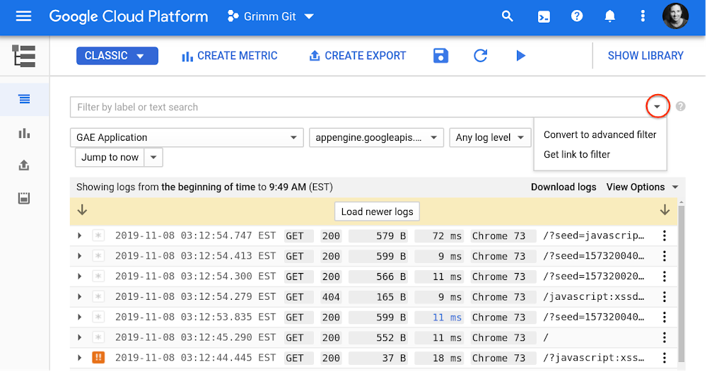
Stackdriver Logging, part of our set of operations management tools at Google Cloud, is designed to manage and analyze logs at scale to help you troubleshoot your hybrid cloud environment and gain insight from your applications. But the sheer volume of machine-generated data can pose a challenge when searching through logs. Through our years of working with Stackdriver Logging users, we’ve identified the easiest ways and best practices to get the value you need from your logs. We’ve collected our favorite tips for more effective log analysis and fast troubleshooting, including a few new features to help you quickly and easily get value from your logs: saved searches, a query library, support for partition tables when exporting logs to BigQuery, and more.1. Take advantage of the advanced query languageThe default basic mode for searching Stackdriver logs is using the drop-down menus to select the resource, log, or severity level. Though this makes it incredibly easy to get started with your logs, most users gravitate toward the advanced filter to ask more complex queries, as shown here:Some powerful tools in this advanced query mode include:Comparison operators:=           # equal!=          # not equal> < >= <=   # numeric ordering:           # “has” matches any substring in the log entry fieldBoolean operators: By default, multiple clauses are combined with AND, though you can also use OR and NOT (be sure to use upper case!)Functions: ip_in_net() is a favorite for analyzing network logs, like this:    ip_in_net(jsonPayload.realClientIP, “10.1.2.0/24″)Pro tip: Include the full log name, time range, and other indexed fields to speed up your search results. See these and other tips on speeding up performance.New queries library: We’ve polled experts from around Google Cloud to collect some of our most common advanced queries by use case including Kubernetes, security, and networking logs, which you can find in a new sample queries library in our documentation. Is there something different you’d like to see? Click the “Send Feedback” button at the top of the Sample Queries page and let us know.2. Customize your search resultsOften there is a specific field buried in your log entries that is of particular interest when you’re analyzing logs. You can customize the search results to include this field by clicking on a field and selecting “Add field to summary line.” You can also manually add, remove, or reorganize fields, or toggle the control limiting their width under View Options. This configuration can dramatically speed up troubleshooting, since you get the necessary context in summary. See an example here:3. Save your favorite searches and custom search results in your personal search libraryWe often hear that you use the same searches over and over again, or that you wish you could save custom field configurations for performing future searches. So, we recently launched a new feature that lets you save your searches, including the custom fields in your own library.You can share your saved searches with users who have permissions on your project by clicking on the selector next to Submit and then Preview. Click the Copy link to filter and share it with your team. This feature is currently in beta, and we’ll continue working on the query library functionality to help you quickly analyze your logs.4. Use logs-based metrics for dashboarding and alertingNow that you’ve mastered advanced queries, you can take your analysis to the next level with real-time monitoring using logs-based metrics. For example, suppose you want to get an alert any time someone grants access to an email address from outside your organization. You can create a metric to match audit logs from Cloud Resource Manager SetIamPolicy calls, where a member not under “my-org.com” domain is granted access, as shown here:With the filter set, simply click Create Metric and give it a name.To alert if a matching log arrives, select Create Alert From Metric from the three-dot menu next to your newly created user-defined metric. This will open a new alerting policy in Stackdriver Monitoring. Change the aggregator to “sum” and the threshold to 0 for “Most recent value” so you’ll be alerted any time a matching log occurs. Don’t worry if there’s no data yet, as your metric will only count log entries since it was created.Additionally, you can add an email address, Slack channel, SMS, or PagerDuty account and name, and save your alerting policy. You can also add these metrics to dashboards along with custom and system metrics.5. Perform faster SQL queries on logs in BigQuery using partitioned tablesStackdriver Logging supports sending logs to BigQuery using log sinks for performing advanced analytics using SQL or joining with other data sources, such as Cloud Billing. We’ve heard from you that it would be easier to analyze logs across multiple days in BigQuery if we supported partitioned tables. So we recently added this partitioned tables option that simplifies SQL queries on logs in BigQuery.When creating a sink to export your logs to BigQuery, you can either use date-sharded tables or partitioned tables. The default selection is a date-sharded table, in which a _YYYYMMDD suffix is added to the table name to create daily tables based on the timestamp in the log entry. Date-sharded tables have a few disadvantages that can add to query overhead:Querying multiple days is harder, as you need to use the UNION operator to simulate partitioning.BigQuery needs to maintain a copy of the schema and metadata for each date-named table.BigQuery might be required to verify permissions for each queried table.When creating a Log Sink, you can now select the Use Partitioned Tables option to make use of partitioned tables in BigQuery to overcome any issues with date-sharded tables.Logs streamed to a partitioned table use the log entry’s timestamp field to write to the correct partition. Queries on such ingestion-time partitioned tables can specify predicate filters on the _PARTITIONTIME or _PARTITIONDATE pseudo column to limit the amount of logs scanned. You can specify a range of dates using a WHERE filter, like this: WHERE _PARTITIONTIME BETWEEN TIMESTAMP(“20191101″) AND TIMESTAMP(“20191105″)Learn more about querying partitioned tables.Find out more about Stackdriver Logging, and join the conversation directly with our engineers and product management team.
Quelle: Google Cloud Platform

Shrinking the time to mitigate production incidents – CRE life lessons

Your pager is going off. Your service is down and your automated recovery processes have failed. You need to get people involved in order to get things fixed. But people are slow to react, have limited expertise, and tend to panic. However, they are your last line of defense, so you’re glad you prepared them for handling this situation.At Google, we follow SRE practices to ensure the reliability of our services, and here on the Customer Reliability Engineering (CRE) team, we share tips and tricks we’ve learned from our experiences helping customers get up and running. If you read our previous post on shrinking the impact of production incidents, you might remember that the time to mitigate an issue (TTM) is the time from when a first responder acknowledges the reception of a page to the time users stop feeling pain from the incident. Today’s post dives deeper into the mitigation phase, focusing on how to train your first responders so they can react efficiently under pressure. You’ll also find templates so you can get started testing these methods in your own organization.Understanding unmanaged vs. untrained responsesEffective incident response and mitigation requires effective technical people and proper incident management. Without it, teams can end up working on fixing technical problems in parallel instead of working together to mitigate the outage. Under these circumstances, actions performed by engineers can potentially worsen the state of the outage, since different groups of people may be undoing each other’s progress. This total lack of incident response management is what we referred to as “unmanaged.”Check out the Site Reliability Workbook for a real example of the consequences of the lack of proper incident management, along with a structure to introduce that incident management to your organization.Solving the problem of the untrained responseWhat we’ll focus on here is the problem that arises when the personnel responding to the outage are managed under a properly established incident response structure, but lack the training to effectively work through the response. In this “untrained” response, the response is coordinated and those responding know and understand their roles, but they lack the technical preparedness to troubleshoot the problem and identify the mitigation path to restore the service. Even if the engineers were once prepared, they can lose their edge if the service has a very low number of pages or if the on-call shifts for an individual are widely spaced in time.Other causes could be fast-paced software development or new service dependencies. Those can lead to the on-call engineers being unfamiliar with the tools and procedures needed to work through an outage. They know what they are supposed to be doing, but they just don’t know how to do it.How can we fix the untrained response to minimize the mean time to mitigation (MTTM)?Teaching response teams with hands-on activitiesThe way humans can cope with sudden changes in the environment, such as those introduced by an emergency, and have a measured response is by establishing mental models that help with pattern recognition. Psychologists call this “expert intuition,” and it helps when identifying underlying commonalities in situations that we have never faced before: “Hmm, I don’t recognize this specifically, but the symptoms we’re seeing make me think of X.”The best way to gain knowledge and, in turn, establish long-term memory and expert intuition, isn’t through one-time viewings of documents or videos. Instead, it’s through a series of exercises that include (but are not limited to) low-stakes struggles. These are situations with never-before-seen (or at least rarely seen) problems, in which failure to solve them will not have a severe impact on your service. These brain challenges help the learning process by practicing memory retrieval and increasing the neuro pathways that access memory, thus improving analytical capacity.At Google, we use two types of exercises to help our learning process: Disaster Recovery Testing (DiRT) and Wheel of Misfortune.DiRT, or how to get dirty The disaster recovery testing we perform internally at Google is a coordinated set of events organized across the company, in which a group of engineers plan and execute real and fictitious outages for a defined period of time to test the effective response of the involved teams. These complex, non-routine outages are performed in a controlled manner, so that they can be rolled back as quickly as possible by the proctors should the tests get out of hand.To ensure consistent behavior across the company, there are some rules of engagement that the coordinating team publishes, and every participating team has to adhere to. These rules include:Prioritizations, i.e., real emergencies take precedence over DiRT exercisesCommunication protocols for the different announcements and global coordinationImpact expectations: “Are services in production expected to be affected?”Test design requirements: all tests must include a revert/rollback plan in case something goes wrongAll tests are reviewed and approved by a cross-functional technical team, different from the coordinating team. One dimension of special interest during this review process is the overall impact of the test. It not only has to be clearly defined, but if there’s a high risk of affecting production services, the test has to be approved by a group of VP-level representatives. It is paramount to understand if a service outage is happening as a direct result of the test being run, or if something is out of control and the test needs to be stopped to fix the unrelated problem.Some examples of practical exercises include disconnecting complete data centers, disruptively diverting the traffic headed to a specific application to a different target, modifying live service configurations, or bringing up services with known bugs. The resilience of the services is also tested by “disabling” people who might have knowledge or experience that isn’t documented, or removing documentation, process elements, or communication channels.Back in the day, Google performed DiRT exercises in a different way, which may be more practical for companies without a dedicated disaster testing team. Initially, DiRT comprised a small set of theoretical tests done by engineers working on user-facing services, and the tests were isolated and very narrow in scope: “What would happen if access to a specific DNS server is down?” or “Is this engineer a single point of failure when trying to bring this service up?”How to start: the basicsOnce you embrace the idea that testing your infrastructure and procedures is a way to learn what works and what does not, and use the failures as a way of growing, it is very tempting to go nuts with your tests. But doing so can easily create too many complications in an already complex system.To avoid the initial unnecessary overhead of interdependencies, start small with service-specific tests, and evolve your exercises, analyzing which ones provide value and which ones don’t. Clearly defining your tests is also important, as it helps to verify if there are hidden dependencies: “Bring down DNS” is not the same as “Shut down all primary DNS servers running in North America data centers, but not the forwarding servers.” Forwarding rules may mask the fact that all the DNS servers are down but the clients are sending DNS queries to external providers.Over the years, your DiRT tests will naturally evolve and increase in size and scope, with the goal of identifying weaknesses in the interfaces between services and teams. This can be achieved, for instance, by failing services in parallel, or by bringing down entire clusters, buildings, geographical domains, cloud zones, network layers, or similar physical or logical groupings.What to test: human learningAs we described earlier, technical knowledge is not everything. Processes and communications are also fundamental in reducing the MTTM. Therefore, DiRT exercises should also test how people organize themselves and interact with each other, and how they use the processes that have previously been established for the resolution of emergencies. It’s not helpful to have a process to purchase fuel for a long-running generator working during an extensive power outage if nobody knows the process exists, or where it is documented.Once you identify failures in your processes, you can put in place a remediation plan. Once the remediation plan has been implemented and a fix is in place, you should make sure the fix is effective by testing it. After that, expand your tests and restart the cycle. If you plan to introduce a DiRT-style exercise in your company, you can use this Test Plan Scenario template to define your tests.Of course, you should note that these exercises can produce accidental user-facing outages, or even revenue loss. During a DiRT exercise, as we are operating on production services, an unknown bug can potentially bring an entire service to a point in which recovery is not automatic, easy, or even documented.We think the learning value of DiRT exercises justifies the cost in the long term, but it’s important to consider whether these exercises might be too disruptive. There are, fortunately, other practices that can be used without creating a major business disruption. Let’s describe the other one we use at Google, and how you can try it.Spinning the Wheel of MisfortuneA Wheel of Misfortune is a role-playing scenario to test techniques for responding to an emergency. The purpose of this exercise is to learn through a purely simulated emergency, using a traditional role-playing setup, where engineers walk through the steps of debugging and troubleshooting. It provides a risk-free environment, where the actions of the engineers will have no effects in production, so that the learning process can be reinforced through low-stakes struggles.The use of scenarios portraying both real and fictitious events also allow the creation of complete operational environments. These scenarios require the use of skills and bits of knowledge that might not be used otherwise, helping the learning process by exposing the engineers to real—but rarely occurring—patterns to help build a complete mental model.If you have played any role-playing game, you probably already know how it works: a leader such as the Dungeon Master, or DM, runs a scenario where some non-player characters get into a situation (in our case, a production emergency) and interact with the players, who are the people playing the role of the emergency responders.Running the scenarioThe DM is generally an experienced engineer who knows how the services work and interact in order to respond to the operations requested by the player(s). It is important that the DM knows what the underlying problem is, and the main path to mitigate its effects. Understanding the information the consoles and dashboards would present, the way the debugging tools work, and the details of their outputs all add realism to the scenario, and will avoid derailing the exercise by providing information and details that are not relevant to the resolution.The exercise usually starts with the DM describing how the player(s) becomes aware of the service breakage: an alert received through a paging device, a call from a call-center support person, an IM from a manager, etc. The information should be complete, and the DM should avoid holding back information that otherwise would be known during the real scenario. Information should also be relayed as it is without any commentary on what it might mean.From there, the player should be driving the scenario: They should give clear explanations of what they want to do, the dashboards they want to visualize, the diagnostic commands they want to run, the config files they want to inspect, and more. The DM in turn should provide answers to those operations, such as the shape of the graphs, the outputs of the different commands, or the content of the files. Screenshots of the different elements (graphs, command outputs, etc.) projected on a screen for everybody to see should be favored over verbal descriptions.It is important for the DM to ask questions like “How would you do that?” or “Where would you expect to find that information?” Exact file system paths or URLs are not required, but it should be evident that the player could find the relevant resource in a real emergency. One option is for the player to do the investigation for real by projecting their laptop screen to the room and looking at the real graphs and logs for the service.In these exercises, it’s important to test not only the players’ knowledge of the systems and their troubleshooting capacity, but also the understanding of incident command procedures. In the case of a large disaster, declaring a major outage and proceeding to identify the incident commander and the rest of the required roles is as important as digging to the bottom of the root cause.The rest of the team should be spectators, unless specifically called in by the DM or the player. However, the DM should exercise veto power for the sake of the learning process. For example, if the player declares the operations lead is another very experienced engineer and calls them in, with the goal of unloading all the troubleshooting operations, the DM could indicate that the experienced engineer is trapped inside a subway car without cell phone reception, and is unable to respond to the call.The DM should be literal in the details: If a page has a three-minute escalation timeout and has not been acknowledged after the timeout, escalate to the secondary. The secondary can be a non-player who then calls the player on the phone to inform them about the page. The DM should also be flexible in the structure. If the scenario is taking too long, or the player is stuck on one part, allow suggestions from the audience, or provide hints through non-player observations.Finally, once the scenario has concluded, the DM should state clearly and affirmatively (if so) that the situation is fixed. Allow some time at the end for debriefing and discussion, explaining the background story that led to the emergency and indicating the contributors to the situation. If the scenario was based on a real outage, the DM can provide some factual details of the context, as they usually help understand the different steps that led to the outage.To make the process of bootstrapping the exercises easier, check out the Wheel of Misfortune template we’ve created that can help you with your Wheel of Misfortune preparation.Putting it all togetherThe people involved in incident response directly affect the time needed to recover from an outage, so it’s important to prepare teams as well as systems. Now that you’ve seen how some testing and learning methods work, try them out for yourself. In the next few weeks, try running a simple Wheel of Misfortune with your team. Choose (or write!) a playbook for an important alert, and walk through it as if you were solving a real incident. You might be amazed at steps that seem obvious that need documenting.Check out these resources to learn more:SRE workbookDisaster Recovery Testing TemplateWheel Of Misfortune Template
Quelle: Google Cloud Platform