Cloud Computing Köln

Gauge the effectiveness of your DevOps organization running in Google Cloud

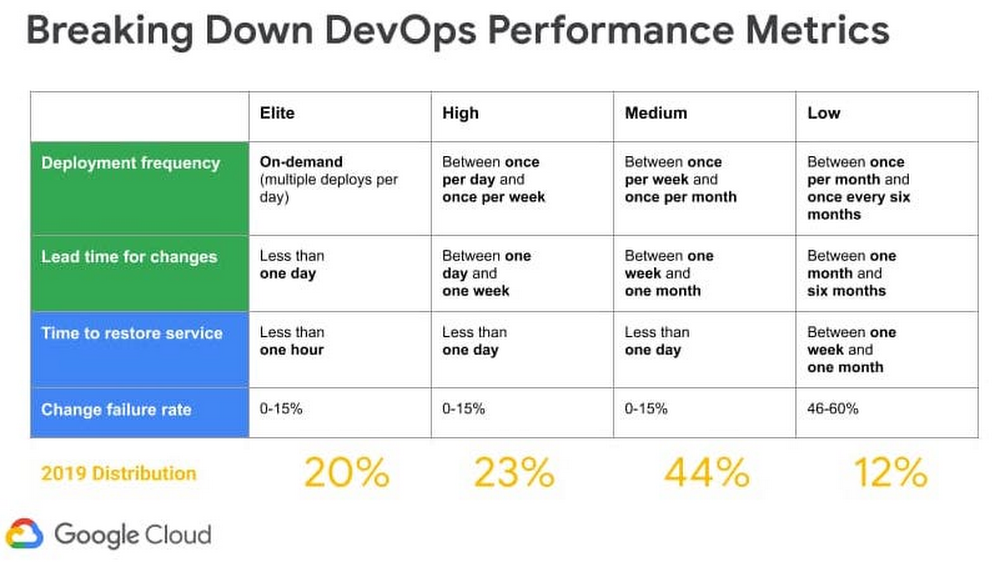
Editor’s note: There are many ways to skin the DevOps cat. Google Cloud Developer Programs Engineer Dina Graves Portman recently wrote about how to evaluate your DevOps effectiveness using the open-source Four Keys project. Here, Google Customer Engineer Brian Kaufman shows you how to do the same thing, but for an application that runs entirely on Google Cloud.Many organizations aspire to become true, high-functioning DevOps shops, but it can be hard to know where you stand. According to DevOps Research and Assessment, or DORA, you can prioritize just four metrics to measure the effectiveness of your DevOps organization—two to measure speed, and two to measure stability:Speed1. Lead Time for Changes – Code commit to code in production2. Deployment Frequency – How often you push codeStability3. Change Failure Rate – Rate of deployment failures in production that require immediate remedy. (Rollback or manual change)4. Time to Restore Service (MTTR) – Mean time to recovery. In this post, we present a methodology to collect these four metrics from software delivery pipelines and applications deployed in Google Cloud. You can then use those metrics to rate your overall practice effectiveness, and baseline your organization’s performance against DORA industry benchmarks, and determine whether you’re an Elite, High, Medium or Low performer.Click to enlargeLet’s take a look at how to do this in practice, with a sample architecture running on Google Cloud. Services and reference architectureTo get started, we create a CI/CD pipeline with the following cloud services: Github Code RepoCloud Build, a container-based CI/CD Tool)Container Registry Google Kubernetes Engine (GKE)Cloud Load Balancing, used as an Ingress Controller for GKE)Cloud Uptime Checks, for synthetic application monitoringCloud MonitoringCloud FunctionsPub/Sub, used as a message bus to connect Alerts to Cloud Functions)These are combined into the reference architecture below. Note that all of these Google Cloud services are integrated with Cloud Monitoring. As such, there’s nothing in particular that you need to set up to receive service logs, and many of these services have built-in metrics that we’ll use in this post.Google Cloud Platform CI/CD pipeline and application topologyMeasuring SpeedTo measure our two speed metrics—deployment frequency and lead time to commit—we instrument Cloud Build, which is a continuous integration and continuous delivery tool. As a container-based CI/CD tool, Cloud Build lets you load a series of Google managed orcommunity managed Cloud Buildersto manipulate your code or interact with internal and external services during the build/deployment process. Upon firing a build trigger, Cloud Build reaches into our Git Repository for our source code, creates a container image artifact that it pushes to the container registry, and then deploys the container image to a GKE cluster.You can also import your own cloud builder container in the process and insert it as the final build step, to determine the time from commit to deployment as well as whether this is a rollback deployment. For this example, we’ve created a custom container to be used as the last build step that:Retrieves the payload binding for the commit timestamp accessed by the variable $(push.repository.pushed_at) and compares it against the current timestamp to calculate lead time. The payload binding variable is used when we create the trigger and is referenced by a custom variable, $_MERGE_TIME in cloudbould.yaml. Reaches into the source repo to get the commit ID of the latest commit on the master branch and compares it to the current commit ID of the build to determine if it is a rollback or a match. You can find a reference Cloud Build config yaml here that shows each build step described above. If you’re using a non-built-in variable like ’$_MERGE_TIME’ payload binding in your config file, you need to specify the variable map when you setup the cloud build trigger to the $(push.repository.pushed_at) value.You can find the custom cloud builder container used here. After the build step for this container runs the following is outputted to the Cloud Build logs, which are fed automatically into Cloud Monitoring. Notice the commit ID, Rollback value, and LeadTime values which are written to the logs from our custom cloud builder:Next we can create a log-based metric in Cloud Logging to absorb these custom values. Log-based metrics can be based on filters for specific log entries.Once we have our specific log entries filter, we can use regular expressions assigned to a particular piece of the output logs to capture specific sections of the log entry into metrics. In the screenshots below we created labels for the commit name and rollback value that will attach to the LeadTime value that shows up in the ‘textPayload’ field of our log. We use the following regular expressions:Metric Value:Create log based metric and labelsLead Time for ChangesOnce we have the above metric and labels created from our Cloud Build log we can access it in Cloud Operations Metrics explorer via the metric label ‘logging/user/dorametics’ (‘DoraMetrics’ was the name we gave our log-based metric). The value of the metric will be the LeadTime as extracted from the regular expression above, with Rollbacks filtered out. We use the median or 50th percentile.Deployment FrequencyNow that we have the lead time for each commit, we can determine the frequency of deployments by just counting the number of lead times we recorded in a window!Measuring stability Change Failure CountTo determine the number of software rollbacks that were performed, we can look at our Deployment Frequency and filter for ‘Rollback=True’ metrics. This gives us a count of the total rollbacks performed. If we wanted to determine the Change Failure Rate we would use data collected in this chart and divide it by the Deployment Frequency metric collected above for the same window.Mean-Time-To-Resolution (MTTR)In typical enterprise environments there are incident response systems that allow you to determine when an issue was reported and when it is ultimately resolved. Assuming these times could be queried, MTTR could be determined by the average time between the reported and resolved timestamps of the issues. In this blog we use automation to alert and graph issues, which allows us to gather more accurate service disruption metrics. Our strategy involves the use of Service Level Objectives (SLO), which represents  Service Level Indicators (SLI)  that we’ve determined represent our customers’ happiness with our application and an objective. When we violate an SLO we consider our mean-time-to-restore service is the total time it takes to detect, mitigate, and resolve a problem until we are back in compliance with the SLO.MTTR and customer satisfactionFor the purposes of simplicity we’ve highlighted one metric we feel represents our customer satisfaction: overall HTTP response code errors from our website. The ratio of this metric against the total response codes sent over a given time window constitutes our Service Level Indicator (SLI). For total errors we monitor response codes returned from our front-end load balancer, which is set up as an ingress controller in our GKE cluster.Metric Used: loadbalancing.googleapis.com/https/request_count Group by response_codeUsing this metric above we can build our SLI and wrap it into an SLO that represents the customer satisfaction observed over a longer time window. Using the SLO API, we create custom SLOs that represent the level of customer satisfaction we want to monitor, where being in violation of that SLO indicates an issue. There’s a great tutorial on how to create custom SLOs and services here. In this example, we’ve created a custom service to represent our application and an SLO for HTTP LB response codes (code). It assumes a quality of service level in which 98% of responses from the load balancer should not be errors in a given day. Doing this automatically creates an error budget of 2% over 24 hours. Now, when it comes to monitoring for MTTR, we have a metric (SLI) that’s attached to a service level SLO that represents quality of service over a given window of time. The failure of the SLO is simulated in the screenshot below:Next, we set up an alert policy that fires when we are in danger of violating this SLO. This also starts a timer to calculate the time-to-resolution. What we’re measuring here is referred to as ‘burn rate’—how much of our error budget (2% of errors over 24 hours) we are eating up with the current SLI metic. The window we measure for our alert is much smaller than our entire SLO so when the SLI has moved back within compliance of a threshold, another alert fires, indicating the incident has cleared. For more information on setting up alerting policies please visit this page. You can also send out alerts through a variety of channels, allowing you to integrate into existing ticketing or messaging systems to record the MTTR in a way that makes sense for your organization. For our purposes we integrate with the Pub/Sub message bus channel, sending the alerts to a cloud function that performs the necessary charting calculators.In the message from the clearing alert we see the JSON payload has the started_at and ended_at timestamps. We use these timestamps in our cloud function to calculate the time to resolve the issue and then output it to the logs.Here is the entire Pub/Sub message sent to Cloud Functions:Here is the cloud function connected to the same Pub/Sub topic as the Alert:The results in the following messages sent to Cloud Functions logs:The final step is to create another log-based metric to pick up the ‘Time to Resolve’ value that we print to our cloud functions log. We do so with this regex expression Resolve:s([0-9]+);Now the metric is available in Cloud Operations.ConclusionWe’ve shown above how you can create custom cloud builders in Cloud Build to generate metrics relating to deployment frequency, mean-time-to-deployment and rollback that will appear in Cloud Operations logs. We’ve also shown you how to use SLOs and SLIs to generate and push alerts to your Cloud Functions logs. We’ve used log-based metrics to pull our metrics out of the logs and chart them. These metrics can be used to evaluate the effectiveness of your organization’s software development and delivery pipelines over time as well as help you evaluate your performance amongst the greater DevOps community. Where does your organization land? For more inspiration, here is some further reference material to help you measure the effectiveness of your own DevOps organization:Google Cloud Application Modernization Program(blog)Setting SLOs: a step-by-step guide (blog)Setting SLOs: observability using custom metrics (blog)Concepts in Service Monitoring(documentation)Working with the SLO API (documentation)How to create SLOs in the GCP Console (video)How to create SLOs at scale with the SLO API (video)How to create SLOs using custom metrics (video)GitHub SLO API Code used for BlogDORA Quick CheckThe 4 Keys Project for DORA Metric Ingression into BigQuery21 new ways we’re improving observability with Cloud Ops (blog)Related ArticleAre you an Elite DevOps performer? Find out with the Four Keys ProjectLearn how the Four Keys open source project lets you gauge your DevOps performance according to DORA metrics.Read Article
Quelle: Google Cloud Platform