A deep dive into Spanner’s query optimizer

Spanner is a fully managed, distributed relational database that provides unlimited scale, global consistency, and up to five 9s availability. It was originally built to address Google’s needs to scale out Online Transaction Processing (OLTP) workloads without losing the benefits of strong consistency and familiar SQL that developers rely on. Today, Cloud Spanner is used in financial services, gaming, retail, health care, and other industries to power mission-critical workloads that need to scale without downtime. Like most modern relational databases, Spanner uses a query optimizer to find efficient execution plans for SQL queries. When a developer or a DBA writes a query in SQL, they describe the results they want to see, rather than how to access or update the data. This declarative approach allows the database to select different query plans depending on a wide variety of signals, such as the size and shape of the data and available indexes. Using these inputs, the query optimizer finds an execution plan for each query.You can see a graphical view of a plan from the Cloud Console. It shows the intermediate steps that Spanner uses to process the query. For each step, it details where time and resources are spent and how many rows each operation produces. This information is useful for identifying bottlenecks and to test changes to queries, indexes, or the query optimizer itself.How does the Spanner query optimizer work?Let’s start with the following example schema and query, using Spanner’s Google Standard SQL dialect. Schema:code_block[StructValue([(u’code’, u’CREATE TABLE Accounts (rn id STRING(MAX) NOT NULL,rn name STRING(MAX) NOT NULL,rn age INT64 NOT NULL,rn) PRIMARY KEY(id);rn rnCREATE INDEX AccountsByName ON Accounts(name);rn rnCREATE TABLE Orders (rn id STRING(MAX) NOT NULL,rn account_id STRING(MAX) NOT NULL,rn date DATE,rn total INT64 NOT NULL,rn) PRIMARY KEY(id);’), (u’language’, u”), (u’caption’, <wagtail.wagtailcore.rich_text.RichText object at 0x3e14c06e31d0>)])]Query:code_block[StructValue([(u’code’, u’SELECT a.id, o.order_idrnFROM Accounts AS a rnJOIN Orders AS o ON a.id = o.account_idrnWHERE a.name = “alice”rn AND o.date = “2022-1-1″;’), (u’language’, u”), (u’caption’, <wagtail.wagtailcore.rich_text.RichText object at 0x3e14ef462f90>)])]When Spanner receives a SQL query, it is parsed into an internal representation known as relational algebra. This is essentially a tree structure in which each node represents some operation of the original SQL. For example, every table access will appear as a leaf node in the tree and every join will be a binary node with its two inputs being the relations that it joins. The relational algebra for our example query looks like this:The query optimizer has two major stages that it uses to generate an efficient execution plan based on this relational algebra: heuristic optimization and cost-based optimization. Heuristic optimization, as the name indicates, applies heuristics, or pre-defined rules, to improve the plan. Those heuristics are manifested in several dozen replacement rules which are a subclass of algebraic transformation rule. Heuristic optimization improves the logical structure of the query in ways that are essentially guaranteed to make the query faster, such as moving filter operations closer to the data they filter, converting outer joins to inner joins where possible, and removing any redundancy in the query. However, many important decisions about an execution plan cannot be made heuristically, so they are made in the second stage, cost-based optimization, in which the query planner uses estimates of latency to choose between available alternatives. Let’s first look at how replacement rules work in heuristic optimization as a prelude to cost-based optimization.A replacement rule has two steps: a pattern matching step and an application step. In the pattern matching step, the rule attempts to match a fragment of the tree with some predefined pattern. When it finds a match, the second step is to replace the matched fragment of the tree with some other predefined fragment of tree. The next section provides a straightforward example of a replacement rule in which a filter operation is moved, or pushed, beneath a join.Example of a replacement ruleThis rule pushes a filer operation closer to the data that it is filtering. The rationale for doing this is two-fold: Pushing filters closer to the relevant data reduces the volume of data to be processed later in the pipelinePlacing a filter closer to the table creates an opportunity to use an index on the filtered column(s) to scan only the rows that qualify the filter.The rule matches the pattern of a filter node with a join node as its child. Details such as table names and the specifics of the filter condition are not part of the pattern matching. The essential elements of the pattern are just the filter with the join beneath it, the two shaded nodes in the tree illustrated below. The two leaf nodes in the picture need not actually be leaf nodes in the real tree, they themselves could be joins or other operations. They are included in the illustration simply to show context.The replacement rule rearranges the tree, as shown below, replacing the filter and join nodes. This changes how the query is executed, but does not change the results. The original filter node is split in two, with each predicate pushed to the relevant sides of the join from which the referenced columns are produced. This tells the query execution to filter the rows before they’re joined, so the join doesn’t have to handle rows that would later be rejected.Cost-based optimizationThere are big decisions about an execution plan for which no effective heuristics exist. These decisions must be made with an understanding of how different alternatives will perform. Hence the second stage of the query optimizer is the cost-based optimizer. In this stage, the optimizer makes decisions based on estimates of the latencies, or the costs, of different alternatives. Cost-based optimization provides a more dynamic approach than heuristics alone. It uses the size and shape of the data to calculate multiple execution plans. To developers, this means more efficient plans out-of-the-box and less hand tuning. The architectural backbone of this stage is the extensible optimizer generator framework known as Cascades. Cascades is the foundation of multiple industry and open-source query optimizers. This optimization stage is where the more impactful decisions are made, such as which indexes to use, what join order to use, and what join algorithms to use. Cost-based optimization in Spanner uses several dozen algebraic transformation rules. However, rather than being replacement rules, they are exploration and implementation rules. These classes of rules have two steps. As for replacement rules, the first step is a pattern matching step. However, rather than replacing the original matched fragment with some fixed alternative fragment, in general they provide multiple alternatives to the original fragment. Example of an exploration ruleThe following exploration rule matches a very simple pattern, a join. It generates one additional alternative in which the inputs to the join have been swapped. Such a transformation doesn’t change the meaning of the query because relational joins are commutative, in much the same way that arithmetic addition is commutative. The content of unshaded nodes in the following illustration do not matter to the rule and they are shown only to provide context.The following tree shows the new fragment that is generated. Specifically, the shaded node below is created as an available alternative to the original shaded node. It does not replace the original node. The unshaded nodes have swapped positions in the new alternative but are not modified in any way. They now have two parents instead of one. At this point, the query is no longer represented as a simple tree but as a directed acyclic graph (DAG). The rationale for this transformation is that the ordering of the inputs to a join can profoundly impact its performance. Typically, a join will perform faster if the first input that it accesses, which for Spanner means left side, is the smaller one. However, the optimal choice will also depend on many other factors, including the available indexes and the ordering requirements of the query.Example of an implementation ruleOnce again the following implementation rule pattern matches a join but this time it generates two alternatives: apply join and hash join. These two alternatives replace the original logical join operation.The above fragment will be replaced by the following two alternatives which are two possible ways of executing a join.Cascades and the evaluation engineThe Cascades engine manages the application of the exploration and implementation rules and all the alternatives they generate. It calls an evaluation engine to estimate the latency of fragments of execution plans and, ultimately, complete execution plans. The final plan that it selects is the plan with the lowest total estimated latency according to the evaluation engine. The optimizer considers many factors when estimating the latency of a node in an execution plan. These include exactly what operation the node performs (e.g. hash join, sort etc.), the storage medium when accessing data, and how the data is partitioned. But chief among those factors is an estimate of how many rows will enter the node and how many rows will exit the node. To estimate those row counts Spanner uses built-in statistics that characterize the actual data.Why does the query optimizer need statistics?How does the query optimizer select which strategies to use in assembling the plan? One important signal is descriptive statistics about the size, shape, and cardinality of the data. As part of regular operation, Spanner periodically samples each database to estimate metrics like distinct values, distributions of values, number of NULLs, data size for each column, and some combination of columns. These metrics are called optimizer statistics.To demonstrate how statistics help the optimizer pick a query plan, let’s consider a simple example using the previously described schema. Let’s look at the optimal plan for this query:code_block[StructValue([(u’code’, u’SELECT id, age FROM Accounts WHERE name = @p’), (u’language’, u”), (u’caption’, <wagtail.wagtailcore.rich_text.RichText object at 0x3e14edfdcf10>)])]There are two possible execution strategies that the query optimizer will consider:Base table plan: read all rows from Accounts and filter out those whose name is different from the value of parameter, @p.Index plan: Read the rows of accounts where name is equal to @p from the AccountsByName index. Then join the set with the Accounts table to fetch the age column.Let’s compare these visually in the plan viewer:Interestingly, even for this simple example there is no query plan that is obviously best. The optimal query plan depends on filter selectivity, or how many rows in Accounts match the condition. For the sake of simplicity let’s suppose that 10 rows in Accounts have name = “alice”, while the remaining 45,000 rows have name = “bob”. The latency of the query with each plan might look something like, using the fastest index plan for alice as our baseline:We can see in this simple example that the optimal query plan choice depends on the actual data stored in the database and the specific conditions in the query, in this example, up to 175 times faster. The statistics describe the shape of data in the database and help Spanner estimate which plan would be preferable for the query.Optimizer statistics collectionSpanner automatically updates the optimizer statistics to reflect the changes to the database schema and data. A background process recalculates them roughly every three days. The query optimizer will automatically use the latest version as input to query planning.In addition to automatic collection, you can also manually refresh the optimizer statistics using the ANALYZE DDL statement. This is particularly useful when a database’s schema or data are changing frequently, such as in a development environment, where you’re changing tables or indexes, or in production when large amounts of data are changing, such as in a new product launch or a large data clean-up. The optimizer statistics include:Approximate number of rows in each table.Approximate number of distinct values of each column and each composite key prefix (including index keys). For example if we have table T with key {a, b, c}, Spanner will store the number of distinct values for {a}, {a, b} and {a, b, c}.Approximate number of NULL, empty and NaN values in each column.Approximate minimum, maximum and average value byte size for each column.Histogram describing data distribution in each column. The histogram captures both ranges of values and frequent values.For example the Accounts table in the previous example has 45,010 total rows. The id column has 45,010 distinct values (since it is a key) and the name column has 2 distinct values (“alice” and “bob”).Histograms store a small sample of the column data to denote the boundaries of histogram bins. Disabling garbage collection for a statistics package will delay wipeout of this data. Query optimizer versioningThe Spanner development team is continuously improving the query optimizer. Each update broadens the class of queries where the optimizer picks the more efficient execution plan. The log of optimizer updates is available in the public documentation.We are doing extensive testing to ensure that new query optimizer versions select better query plans than before. Because of this, most workloads should not have to worry about query optimizer rollouts. By staying current they automatically inherit improvements as we enable them.There is a small chance, however, that an optimizer update will flip a query plan to a less performant one. If this happens, it will show up as a latency increase for the workload. Cloud Spanner provides several tools for customers to address this risk.Spanner users can choose which optimizer version to use for their queries. Databases use the newest optimizer by default. Spanner allows users to override the default query optimizer version through database options or set the desired optimizer version for each individual query.New optimizer versions are released as off-by-default for at least 30 days. You can track optimizer releases in the public Spanner release notes. After that, the new optimizer version is enabled by default. This period offers an opportunity to test queries against the new version to detect any regressions. In the rare cases that the new optimizer version selects suboptimal plans for critical SQL queries, you should use query hints to guide the optimizer. You can also pin a database or an individual query to the older query optimizer, allowing you to use older plans for specific queries, while still taking advantage of the latest optimizer for most queries. Pinning optimizer and statistics versions allows you to ensure plan stability to predictably rollout changes.In Spanner the query plan will not change as long the queries are configured to use the same optimizer version and rely on the same optimizer statistics. Users wishing to ensure that execution plans for their queries do not change can pin both the optimizer version and the optimizer statistics.To pin all queries against a database to an older optimizer version (e.g. version 4), you can set a database option via DDL:code_block[StructValue([(u’code’, u’ALTER DATABASE MyDatabase SET OPTIONS (optimizer_version = 4);’), (u’language’, u”), (u’caption’, <wagtail.wagtailcore.rich_text.RichText object at 0x3e14edff4350>)])]Spanner also provides a hint to more surgically pin a specific query. For example:code_block[StructValue([(u’code’, u’@{OPTIMIZER_VERSION=4} SELECT * FROM Accounts;’), (u’language’, u”), (u’caption’, <wagtail.wagtailcore.rich_text.RichText object at 0x3e14b7cf5fd0>)])]The Spanner documentation provides detailed strategies for managing the query optimizer version. Optimizer statistics versioningIn addition to controlling the version of the query optimizer, Spanner users can also choose which optimizer statistics will be used for the optimizer cost model. Spanner stores the last 30 days worth of optimizer statistics packages. Similarly to the optimizer version, the latest statistics package is used by default, and users can change it at a database or query level.Users can list the available statistics packages with this SQL query:code_block[StructValue([(u’code’, u’SELECT * FROM INFORMATION_SCHEMA.SPANNER_STATISTICS’), (u’language’, u”), (u’caption’, <wagtail.wagtailcore.rich_text.RichText object at 0x3e14b7cf54d0>)])]To use a particular statistics package it first needs to be excluded from garbage collection.code_block[StructValue([(u’code’, u’ALTER STATISTICS <package_name> SET OPTIONS (allow_gc=false);’), (u’language’, u”), (u’caption’, <wagtail.wagtailcore.rich_text.RichText object at 0x3e14ec3b7d50>)])]Then to use the statistics package by default for all queries against a database:code_block[StructValue([(u’code’, u’ALTER DATABASE <db>rnSET OPTIONS (optimizer_statistics_package = “<package name>”);’), (u’language’, u”), (u’caption’, <wagtail.wagtailcore.rich_text.RichText object at 0x3e14c01e5950>)])]Like the optimizer version above, you can also use a hint to pin the statistics package for an individual query using a hint:code_block[StructValue([(u’code’, u’@{OPTIMIZER_STATISTICS_PACKAGE=<package name>} SELECT * FROM Accounts;’), (u’language’, u”), (u’caption’, <wagtail.wagtailcore.rich_text.RichText object at 0x3e14c0f13b10>)])]Get started todayGoogle is continuously improving out-of-the-box performance of Spanner and reducing the need for manual tuning. The Spanner query optimizer uses multiple strategies to generate query plans that are efficient and performant. In addition to a variety of heuristics, Spanner uses true cost-based optimization to evaluate alternative plans and select the one with the lowest latency cost. To estimate these costs, Spanner automatically tracks statistics about the size and shape of the data, allowing the optimizer to adapt as schemas, indexes, and data change. To ensure plan stability, you can pin the optimizer version or the statistics that it uses at the database or query level. Learn more about the query optimizer or try out Spanner’s unmatched availability and consistency at any scale today for free for 90 days or as low as $65 USD per month.
Quelle: Google Cloud Platform

Building advanced Beam pipelines in Scala with SCIO

Apache Beam is an open source, unified programming model with a set of language-specific SDKs for defining and executing data processing workflows. Scio, pronounced shee-o, is Scala API for Beam developed by Spotify to build both Batch and Streaming pipelines. In this blog we will uncover the need for SCIO and a few reference patterns.Why ScioSCIO provides high level abstraction for developers and is preferred for following reasons:Striking balance between concise and performance. Pipeline written in Scala are concise compared to java with similar performanceEasier migration for Scalding/Spark developers due to similar semantics compared to Beam API thereby avoiding a steep learning curve for developers.Enables access to a large ecosystem of infrastructure libraries in Java e.g. Hadoop, Avro, Parquet and high level numerical processing libraries in Scala like Algebirdand Breeze.Supports Interactive exploration of data and code snippets using SCIO REPLReference Patterns Let us checkout few concepts along with examples: 1. Graph CompositionIf you have a complex pipeline consisting of several transforms, the feasible approach is to compose the logically related transforms into blocks.  This would make it easy to manage and debug the graph rendered on dataflow UI. Let us consider an example using popular WordCount pipeline. Fig:  Word Count Pipeline without Graph Composition Let us modify the code to group the related transforms into blocks:Fig:  Word Count Pipeline with Graph Composition2. Distributed CacheDistributed Cache allows to load the data from a given URI on workers and use the corresponding data across all tasks (DoFn’s) executing on the worker. Some of the common use cases are loading serialized machine learning model from object stores like Google Cloud Storage for running predictions,  lookup data references etc.Let us checkout an example that loads lookup data from CSV file on worker during initialization and utilizes to count the number of matching lookups for each input element.Fig:  Example demonstrating Distribute Cache3. Scio JoinsJoins in Beam are expressed using CoGroupByKey  while Scio allows to express various join types like inner, left outer and full outer joins through flattening the CoGbkResult. Hash joins (syntactic sugar over a beam side input) can be used, if one of the dataset is extremely small (max ~1GB) by representing a smaller dataset on the right hand side. Side inputs are small, in-memory data structures that are replicated to all workers and avoids shuffling. MultiJoin can be used to join up to 22 data sets. It is recommended that all data sets be ordered in descending size, because non-shuffle joins do require the largest data sets to be on the left of any chain of operators Sparse Joins can be used for cases where the left collection (LHS) is much larger than the right collection (RHS) that cannot fit in memory but contains a sparse intersection of keys matching with the left collection .  Sparse Joins are implemented by constructing a Bloom filter of keys from the right collection and split the left side collection into 2 partitions. Only the partition with keys in the filter go through the join and the rest are either concatenated (i.e Outer join) or discarded (Inner join). Sparse Join is especially useful for joining historical aggregates with incremental updates.Skewed Joins are a more appropriate choice for cases where the left collection (LHS) is much larger and contains hotkeys.  Skewed join uses Count Mink Sketch which is a probabilistic data structure to count the frequency of keys in the LHS collection.  LHS is partitioned into Hot and chill partitions.  While the Hot partition is joined with corresponding keys on RHS using a Hash join, chill partition uses a regular join and finally both the partitions are combined through union operation.Fig:  Example demonstrating Scio JoinsNote that while using Beam Java SDK you can also take advantage of some of the similar join abstractions using Join Library extension4. AlgeBird Aggregators and SemiGroupAlgebird is Twitter’s abstract algebra library containing several reusable modules for parallel aggregation and approximation. Algebird Aggregator or Semigroup can be used with aggregate and sum transforms on SCollection[T] or aggregateByKey and sumByKey transforms on SCollection[(K, V)].  Below example illustrates computing parallel aggregation on customer orders and composition of result into OrderMetrics classFig:  Example demonstrating Algebird Aggregators Below code snippet expands on previous example and demonstrates the SemiGroup for aggregation of objects by combining fields.Fig:  Example demonstrating Algebird SemiGroup5. GroupMap and GroupMapReduceGroupMap can be used as a replacement of groupBy(key) + mapValues(_.map(func)) or _.map(e  => kv.of(keyfunc, valuefunc)) + groupBy(key)Let us consider the below example that calculates the length of words for each type. Instead of grouping by each type and applying length function, the GroupMap allows combining these operations by applying keyfunc and valuefunc. Fig:  Example demonstrating GroupMapGroupMapReduce  can be used to derive the key and apply the associative operation on the values associated with each key. The associative function is performed locally on each mapper similarly to a “combiner” in MapReduce (aka combiner lifting) before sending the results to the reducer.  This is equivalent to keyBy(keyfunc) + reduceByKey(reducefunc) Let us consider the below example that calculates the cumulative sum of odd and even numbers in a given range.  In this case individual values are combined on each worker and the local results are aggregated to calculate the final resultFig:  Example demonstrating GroupMapReduceConclusionThanks for reading and I hope now you are motivated to learn more about SCIO.  Beyond the patterns covered above, SCIO contains several interesting features likeimplicit coders for Scala case classes,  Chaining jobs using I/O Taps , Distinct Count using HyperLogLog++ , Writing sorted output to files etc.  Several use case specific libraries like BigDiffy (comparison of large datasets) , FeaTran (used for ML Feature Engineering) were also built on top of SCIO. For Beam lovers with Scala background, SCIO is the perfect recipe for building complex distributed data pipelines.
Quelle: Google Cloud Platform

Built with BigQuery: How True Fit's data journey unlocks partner growth

Editor’s note: The post is part of a series highlighting our awesome partners, and their solutions, that are Built with BigQuery.“True Fit is in a unique position where we help shoppers find the right sizes of apparel and footwear through near real time, adaptable ML models thereby rendering a great shopping experience while also enabling retailers with higher conversion, revenue potential and more importantly access to actionable key business metrics. Our ability to process volumes of data, adapt our core ML models, reduce complex & slower ecosystems, exchange data easily with our customers etc, have been propelled multi-fold via BigQuery and Analytics Hub” – says Raj Chandrasekaran, CTO, True FitTrue Fit has built the world’s largest dataset for apparel and footwear retailers over the last twelve years, connecting purchasing and preference information for more than 80 million active shoppers to data for 17,000 brands across its global network of retail partners. This dataset powers fit personalization for shoppers as they buy apparel and footwear online and connects retailers with powerful data and insight to inform marketing, merchandising, product development and ecommerce strategy.Gathering data, correlating and analyzing it are the underlying foundation to making smart business decisions to grow and scale a retailer’s business. This is especially important for retailers that are utilizing data packages to target which consumers to market their brands and products to. Deriving meaningful insights from data has become a larger focus for retailers as the market grows digitally, competition for share of wallet increases and consumer expectations for more personalized  shopping experiences continues to rise.But, how do companies share datasets regardless of the magnitude amongst each other in a scalable manner by optimizing infrastructure costs and securely sharing data? How can companies access and use the data into their own environment without needing a complicated / time consuming process to physically move the data? How would a company know how to utilize this data to suit their own business needs? True Fit partnered with Google and the Built with BigQuery initiative to solve these questions.Google Cloud services such as BigQuery and Analytics Hub have become vital to how True Fit optimizes the entire lifecycle of data from ingestion to distribution of data packages with its retail partners. BigQuery is a fully managed, serverless and limitless scale data warehousing solution with tighter integration with several Google Cloud products. Analytics Hub, powered by BigQuery, allows easy creation of data exchanges for producers and simplifies the discovery and consumption of the data for the consumers. Data shared via the exchanges can further be enriched with more datasets available in the Analytics Hub marketplace.Using the above diagram, let us take a look at how the process works across different stages:Event Ingestion – True Fit leverages Cloud Logging with Fluentd to stream logging events into BigQuery as datasets. BigQuery’s unique capability in real time streaming allows for real time debugging and analysis of all activity across the True Fit ecosystem.Denormalization – Scheduled queries are set up to take the normalized data in the event logs and convert them into denormalized core tables. These tables are easy to query and contain all information needed to assist BI analysts and data scientists with their research without the need for complicated table joins.Aggregations – Aggregations are created and updated on the fly as data is ingested using a mix of scheduled queries and direct BigQuery table updates. Reports are always fresh and can be delivered without ever having to worry about stale data.Alerting – Alerts are set up all across the True Fit architecture which leverage the real-time aggregations. These alerts not only inform True Fit when there are data discrepancies or missing data but have also been configured to inform our partners when the data they provide contains errors. For example, True Fit will notify a retailer if the product catalog provided drops below specific thresholds we’ve previously seen from them. Alerts range from anything like an email, SMS message, or even a real-time toast message in a True Fit UI that a retailer is using to provide their data.Secure Distribution – Exchange’s are created in the Analytics Hub. The datasets are published as one or more listings into the Exchange. Partners subscribe to the listing as a linked dataset to get instant access to data and act upon it accordingly. This unlocks use cases that range from everywhere from marketing; to shopper chat bots; and even real-time product recommendations based on a shopper’s browsing behavior. Analytics Hub allows True Fit to expose only the data they intend to share to specific partners using simple to understand IAM roles. Adding the built-in Analytics Hub Subscriber role to a partner’s service account on a specific listing of dataset created just for them makes it so that they are the only one to get access to that data. Gone are the days of dealing with API keys or credential management!True Fit’s original data lake was built using Apache Hive prior to switching to BigQuery. At roughly 450TiB, extracting data from this data lake became quite a challenge to do in real-time. It took approximately 24 hours before data packages would become available to core retail partners which impacted our ability to produce reports and data packages at scale. Even after the data packages were available, partners had difficulty downloading these data packages and importing them into their own data warehouses to utilize due to the size and formats. The usefulness of the data packages would occasionally get put into question due to the data becoming stale and it was difficult to alert on any data discrepancies because of the time delay before these data packages would be available.BigQuery has allowed True Fit to produce these same data packages in real time as events occur; unlocking new marketing opportunities. Retail partners have also praised how easily consumable Analytics Hub has made the process because the data “just appears” alongside their existing data warehouse as linked datasets. True Fit publishes a number of BigQuery data packages for its retail partners via Analytics Hub which allows them to generate personalized onsite and email campaigns for their own shoppers in a manner far beyond the capabilities not available in the past. Below are just a sample of ways in which True Fit partners personalize their campaigns utilizing the True Fit data packages. Partners have the ability to:Find the True Fit shoppers of a desired category near real-time who’ve been browsing extra specific products in the last couple weeksEnhance their understanding of their shopper demographic data and category affinitiesRetrieve size and fit recommendations for specific in-stock products for a provided set of shoppers or have True Fit determine what the ideal set of shoppers for those products would beMatch their in-stock, limited run styles and sizes to applicable True Fit shoppersEnhance emails and on-site triggers based on products the shopper has recently viewed or purchased across the True Fit networkIf you’re a retailer looking to unlock your own growth using real-world data in real-time, be sure to check out the data packages offered by True Fit!To learn more about True Fit on Google Cloud, visit https://www.truefit.com/businessThe Built with BigQuery advantage for ISVs Through the Built with BigQuery Program launched in April ‘22 as part of the Google Data Cloud Summit, Google is helping data-driven companies like True Fit build innovative applications on Google’s data cloud with simplified access to technology, helpful and dedicated engineering support, and joint go-to-market programs. Participating companies can: Get started fast with a Google-funded, pre-configured sandbox. Accelerate product design and architecture through access to designated experts from the ISV Center of Excellence who can provide insight into key use cases, architectural patterns, and best practices. Amplify success with joint marketing programs to drive awareness, generate demand, and increase adoption.BigQuery gives ISVs the advantage of a powerful, highly scalable data warehouse that’s integrated with Google Cloud’s open, secure, sustainable platform. And with a huge partner ecosystem and support for multi-cloud, open source tools, and APIs, Google provides technology companies the portability and extensibility they need to avoid data lock-in.Click here to learn more about Built with BigQuery.We thank the many Google Cloud and True Fit team members who contributed to this ongoing collaboration and review, especially Raj Chandrasekaran, CTO True Fit and Sujit Khasnis, Cloud Partner Engineering
Quelle: Google Cloud Platform

Sharing the latest improvements to efficiency in Microsoft’s datacenters

In April, I published a blog that explained how we define and measure energy and water use at our datacenters, and how we are committed to continuous improvements.

Now, in the lead up to COP27, the global climate conference to be held in Egypt, I am pleased to provide a number of updates on how we’re progressing in making our datacenters more efficient across areas such as waste, renewables, and ecosystems. You can also visit Azure Sustainability—Sustainable Technologies | Microsoft Azure to explore this further.

Localized fact sheets in 28 regions

To share important information about the impact of our datacenters regionally with our customers, we have published localized fact sheets in 28 regions across the globe. These fact sheets provide a wide range of information and details about many different aspects of our datacenters and their operations.

A review of PUE (Power Usage Effectiveness) and WUE (Water Usage Effectiveness)

PUE is an industry metric that measures how efficiently a datacenter consumes and uses the energy that powers a datacenter, including the operation of systems like powering, cooling, and operating the servers, data networks and lights. The closer the PUE number is to “1,” the more efficient the use of energy.
While local environment and infrastructure can affect how PUE is calculated, there are also slight variations across providers.

Here is the simplest way to think about PUE:

WUE is another key metric relating to the efficient and sustainable operations of our datacenters and is a crucial aspect as we work towards our commitment to be water positive by 2030. WUE is calculated by dividing the number of liters of water used for humidification and cooling by the total annual amount of power (measured in kWh) needed to operate our datacenter IT equipment.

In addition to PUE and WUE, below are key highlights across carbon, water, and waste initiatives at our datacenters.

Datacenter efficiency in North and South America

As I illustrated in April, our newest generation of datacenters have a design PUE of 1.12; this includes our Chile datacenter that is under construction. We are constantly focused on improving our energy efficiency, for example in California, our San Jose datacenters will be cooled with an indirect evaporative cooling system using reclaimed water all year and zero fresh water. Because the new datacenter facilities will be cooled with reclaimed water, they will have a WUE of 0.00 L/kWh in terms of freshwater usage.

In addition, as we continue our journey to achieve zero waste by 2030, we are proud of the progress we are making with our Microsoft Circular Centers. These centers sit adjacent to a Microsoft datacenter and process decommissioned cloud servers and hardware. Our teams sort and intelligently channel the components and equipment to optimize, reuse or repurpose.

In October, we launched a Circular Center in Chicago, Illinois that has the potential capacity to process up to 12,000 servers per month for reuse, diverting up to 144,000 servers annually. We plan to open a Circular Center in Washington state early next year and have plans for Circular Centers in Texas, Iowa, and Arizona to further optimize our supply chain and reduce waste.

Furthermore, our team has successfully completed an important water reuse project at one of our datacenters. This treatment facility, the first of its kind in Washington state and over 10 years in the making, will process water for reuse by local industries, including datacenters, decreasing the need for potable water for datacenter cooling.

Innovative solutions in Europe, the Middle East, and Africa

This winter Europeans face the possibility of an energy crisis, and we have made a number of investments in optimizing energy efficiency in our datacenters to ensure that we are operating our facilities as effectively as possible. Datacenters are the backbone of modern society and as such it is important that we continue to provide critical services to the industries that need us most in a way that constantly mitigates energy consumption.

Across our datacenters in EMEA, we have made steady progress across carbon, waste, water, and ecosystems. We are committed to shifting to 100 percent renewable energy supply by 2025, meaning that we will have power purchase agreements for green energy contracted for 100 percent of carbon emitting electricity consumed by all our data centers, buildings, and campuses. This will add additional gigawatts of renewable energy to the grid, increasing energy capacity. With that said we have added more than 5 gigawatts of renewable energy to the grid globally, this has culminated in more than 15 individuals deals in Europe spanning Ireland, Denmark, Sweden, and Spain.

In Finland, we recently announced an important heat reuse project that will take excess heat from our datacenters and transfer that heat to the local districts’ heating systems that can be used for both domestic and commercial purposes.

To reduce waste from our datacenters in EMEA, the Circular Center we opened in Amsterdam in 2020, which has since already delivered an 83 percent reuse of end-of-life datacenter assets and components. This is progress towards our target of 90 percent reuse and recycling of all servers and components for all cloud hardware by 2025. In addition, in January 2022, we opened a Circular Center in Dublin, Ireland, and have plans to open another Circular Center in Sweden to serve the region.

As we continue to seek out efficiencies in our operations, recently we turned to nature for inspiration, to understand how much of the natural ecosystem we could replenish on the site of a datacenter, essentially integrating the datacenter into nature with the goal of renewing and revitalizing the surrounding area so that we can restore and create a pathway to provide regenerative value for the local community and environment. In the Netherlands we have begun construction of a lowland forested area around the datacenter as well as forested wetland. This was done to support the growth of native plants to mirror a healthy, resilient ecosystem and support biodiversity, improve storm water control and prevent erosion.

Updates in Asia Pacific

Finally, I’d like to highlight some of the sustainability investments we have made across Asia Pacific. In June 2022, we launched our Singapore Circular Center that is capable of processing up to 3,000 servers per month for reuse, or 36,000 servers annually. We have plans to open additional Circular Centers in Australia and South Korea in fiscal year 2025 and beyond. Across our datacenters in APAC, we have formed partnerships with local energy providers for renewable energy that is sourced from wind, solar, and hydro power and we have plans to further these partnerships and investments in renewable energy. In our forthcoming datacenter region in New Zealand, we have signed an agreement that will enable Microsoft to power all of its datacenters with 100 percent renewable energy from the day it opens.

Innovating to design the hyperscale datacenter of the future

What these examples from across our global datacenter portfolio show is our ongoing commitment to make our global Microsoft datacenters more sustainable and efficient, enabling our customers to do more with less.

Our objective moving forward is to continue providing transparency across the entire datacenter lifecycle about how we infuse principles of reliability, sustainability, and innovation at each step of the datacenter design, construction, and operations process.

Design: How do we ensure we design for reliability, efficiency, and sustainability, to help reduce our customers' scope three emissions?
Construction: How do we reduce embodied carbon and create a reliable supply chain?
Operation: How do we infuse innovative green technologies to decarbonize and operate to the efficient design standards?
Decommissioning: How do we recycle and reuse materials in our datacenters?
Community: How do we partner with the community and operate as good neighbors?

We have started by sharing datacenter region-specific data around carbon, water, waste, ecosystems, and community development and we will continue to provide updates as Microsoft makes further investments globally.

Learn more

You can learn more about our global datacenter footprint across the 60+ datacenter regions by visiting datacenters.microsoft.com.

View our Microsoft datacenter factsheets.
Learn more about Azure sustainability.
Discover new sustainability guidance in the Azure Well-Architected Framework.
Take a virtual tour of Microsoft’s datacenters.

Quelle: Azure

Build a globally resilient architecture with Azure Load Balancer

Azure Load Balancer’s global tier is a cloud-native global network load balancing solution. With cross-region Load Balancer, customers can distribute traffic across multiple Azure regions with ultra-low latency and high performance. To better understand the use case of Azure’s cross-region Load Balancer, let’s dive deeper into a customer scenario. In this blog, we’ll learn about a customer, their use case, and how Azure Load Balancer came to the rescue.

Who can benefit from Azure Load Balancer?

This example customer is a software vendor in the automotive industry. Their current product offerings are cloud–based software, focused on helping vehicle dealerships manage all aspects of their business including sales leads, vehicles, and customer accounts. While it is a global company, most of its business is done in Europe, the United Kingdom (UK), and Asia Pacific regions. To support its global business, the customer utilizes a wide range of Azure services including virtual machines (VMs), a variety of platform as a service (PaaS) solutions, Load Balancer, and MySQL to help meet an ever-growing demand.

What are the current global load balancing solutions?

The customer is using domain name service (DNS)–based traffic distribution to direct traffic to multiple Azure regions. At each Azure region, they deploy regional Azure Load Balancers to distribute traffic across a set of virtual machines. However, if a region went down, they experienced downtime due to DNS caching. Although minimal, this was not a risk they could continue to take on as their business expanded globally.

What are the problems with the current solutions?

Since the customer’s solution is global, as traffic increased, they noticed high latency when requesting information from their endpoints across regions. For example, users located in Africa noticed high latency when they tried to request information. Often their requests were routed to an Azure region on another continent, which caused the high latency. Answering requests with low latency is a critical business requirement to ensure business continuity. As a result, they needed a solution that withstood regional failover, while simultaneously providing ultra-low latency with high performance.

How did Azure’s cross-region Load Balancer help?

Given that low latency is a requirement for the customer, a global layer 4 load balancer was a perfect solution to the problem. The customer deployed Azure’s cross-region Load Balancer, giving them a single unique globally anycast IP to load balance across their regional offices. With Azure’s cross-region Load Balancer, traffic is distributed to the closest region, ensuring low latency when using the service. For example, if a customer connected from Asia Pacific regions, traffic is automatically routed to the closest region, in this case Southeast Asia. The customer was able to add all their regional load balancers to the backend of the cross-region Load Balancer and thus improved latency without any additional downtime. Before the update was deployed across all regions, the customer verified that their metrics for data path availability and health probe status are 100 percent on both its cross-region Load Balancer and each regional Load Balancer.
 

After deploying cross-region Load Balancer, traffic is now distributed with ultra-low latency across regions. Since the cross-region Load Balancer is a network load balancer, only the TCP/UDP headers are quickly inspected instead of the entire packet. In addition, the cross-region Load Balancer will send traffic to the closest participating Azure region to a client. These benefits are seen by the customer who now sees traffic being served with lower latency than before.

Learn More

Visit the Cross-region load balancer overview to learn more about Azure’s cross-region Load Balancer and how it can fit into your architecture.
Quelle: Azure

Developing Go Apps With Docker

Go (or Golang) is one of the most loved and wanted programming languages, according to Stack Overflow’s 2022 Developer Survey. Thanks to its smaller binary sizes vs. many other languages, developers often use Go for containerized application development. 

Mohammad Quanit explored the connection between Docker and Go during his Community All-Hands session. Mohammad shared how to Dockerize a basic Go application while exploring each core component involved in the process: 

Follow along as we dive into these containerization steps. We’ll explore using a Go application with an HTTP web server — plus key best practices, optimization tips, and ways to bolster security. 

Go application components

Creating a full-fledged Go application requires you to create some Go-specific components. These are essential to many Go projects, and the containerization process relies equally heavily on them. Let’s take a closer look at those now. 

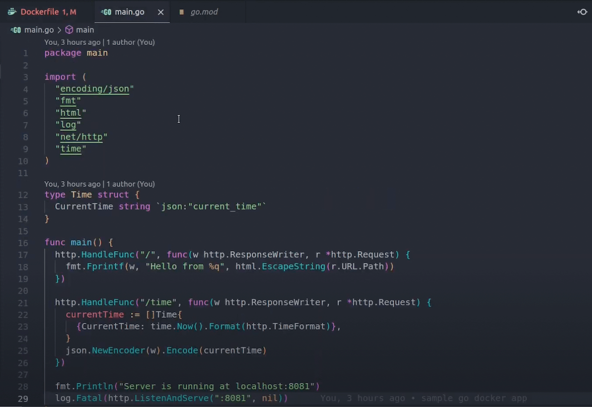
Using main.go and go.mod

Mohammad mainly highlights the main.go file since you can’t run an app without executable code. In Mohammad’s case, he created a simple web server with two unique routes: an I/O format with print functionality, and one that returns the current time.

What’s nice about Mohammad’s example is that it isn’t too lengthy or complex. You can emulate this while creating your own web server or use it as a stepping stone for more customization.

Note: You might also use a package main in place of a main.go file. You don’t explicitly need main.go specified for a web server — since you can name the file anything you want — but you do need a func main () defined within your code. This exists in our sample above.

We always recommend confirming that your code works as expected. Enter the command go run main.go to spin up your application. You can alternatively replace main.go with your file’s specific name. Then, open your browser and visit http://localhost:8081 to view your “Hello World” message or equivalent. Since we have two routes, navigating to http://localhost:8081/time displays the current time thanks to Mohammad’s second function. 

Next, we have the go.mod file. You’ll use this as a root file for your Go packages, module path for imports (shown above), and for dependency requirements. Go modules also help you choose a directory for your project code. 

With these two pieces in place, you’re ready to create your Dockerfile! 

Creating your Dockerfile

Building and deploying your Dockerized Go application means starting with a software image. While you can pull this directly from Docker Hub (using the CLI), beginning with a Dockerfile gives you more configuration flexibility. 

You can create this file within your favorite editor, like VS Code. We recommend VS Code since it supports the official Docker extension. This extension supports debugging, autocompletion, and easy project file navigation. 

Choosing a base image and including your application code is pretty straightforward. Since Mohammad is using Go, he kicked off his Dockerfile by specifying the golang Docker Official Image as a parent image. Docker will build your final container image from this. 

You can choose whatever version you’d like, but a pinned version like golang:1.19.2-bullseye is both stable and slim. Newer image versions like these are also safe from October 2022’s Text4Shell vulnerability. 

You’ll also need to do the following within your Dockerfile: 

Include an app directory for your source codeCopy everything from the root directory into your app directoryCopy your Go files into your app directory and install dependenciesBuild your app with configurationTell your Docker container to listen on a certain port at runtimeDefine an executable command that runs once your container starts

With these points in mind, here’s how Mohammad structured his basic Dockerfile:

# Specifies a parent image
FROM golang:1.19.2-bullseye

# Creates an app directory to hold your app’s source code
WORKDIR /app

# Copies everything from your root directory into /app
COPY . .

# Installs Go dependencies
RUN go mod download

# Builds your app with optional configuration
RUN go build -o /godocker

# Tells Docker which network port your container listens on
EXPOSE 8080

# Specifies the executable command that runs when the container starts
CMD [ “/godocker” ]

From here, you can run a quick CLI command to build your image from this file: 

docker build –rm -t [YOUR IMAGE NAME]:alpha .

This creates an image while removing any intermediate containers created with each image layer (or step) throughout the build process. You’re also tagging your image with a name for easier reference later on. 

Confirm that Docker built your image successfully by running the docker image ls command:

If you’ve already pulled or built images in the past and kept them, they’ll also appear in your CLI output. However, you can see Mohammad’s go-docker image listed at the top since it’s the most recent. 

Making changes for production workloads

What if you want to account for code or dependency changes that’ll inevitably occur with a production Go application? You’ll need to tweak your original Dockerfile and add some instructions, according to Mohammad, so that changes are visible and the build process succeeds:

FROM golang:1.19.2-bullseye

WORKDIR /app

# Effectively tracks changes within your go.mod file
COPY go.mod .

RUN go mod download

# Copies your source code into the app directory
COPY main.go .

RUN go mod -o /godocker

EXPOSE 8080

CMD [ “/godocker” ]

After making those changes, you’ll want to run the same docker build and docker image ls commands. Now, it’s time to run your new image! Enter the following command to start a container from your image: 

docker run -d -p 8080:8081 –name go-docker-app [YOUR IMAGE NAME]:alpha

Confirm that this worked by entering the docker ps command, which generates a list of your containers. If you have Docker Desktop installed, you can also visit the Containers tab from the Docker Dashboard and locate your new container in the list. This also applies to your image builds — instead using the Images tab. 

Congratulations! By tracing Mohammad’s steps, you’ve successfully containerized a functioning Go application. 

Best practices and optimizations

While our Go application gets the job done, Mohammad’s final image is pretty large at 913MB. The client (or end user) shouldn’t have to download such a hefty file. 

Mohammad recommends using a multi-stage build to only copy forward the components you need between image layers. Although we start with a golang:version as a builder image, defining a second build stage and choosing a slim alternative like alpine helps reduce image size. You can watch his step-by-step approach to tackling this. 

This is beneficial and common across numerous use cases. However, you can take things a step further by using FROM scratch in your multi-stage builds. This empty file is the smallest we offer and accepts static binaries as executables — making it perfect for Go application development. 

You can learn more about our scratch image on Docker Hub. Despite being on Hub, you can only add scratch directly into your Dockerfile instead of pulling it. 

Develop your Go application today

Mohammad Quanit outlined some user-friendly development workflows that can benefit both newer and experienced Go users. By following his steps and best practices, it’s possible to create cross-platform Go apps that are slim and performant. Docker and Go inherently mesh well together, and we also encourage you to explore what’s possible through containerization. 

Want to learn more?

Check out our Go language-specific guide.Read about the golang Docker Official Image.See Go in action alongside other technologies in our Awesome Compose repo.Dig deeper into Dockerfile fundamentals and best practices.Understand how to use Go-based server technologies like Caddy 2.
Quelle: https://blog.docker.com/feed/

AWS Global Accelerator kündigt AddEndpoints- und RemoveEndpoints-APIs an

AWS Global Accelerator bietet jetzt zwei neue APIs, AddEndpoints und RemoveEndpoints, mit denen Sie Endpunkte hinter Ihrem Accelerator hinzufügen und entfernen können. Mit diesen neuen APIs können Sie jetzt Endpunkte hinter Ihren Accelerators konfigurieren, ohne zum Hinzufügen oder Entfernen von Endpunkten die vollständige Liste der Endpunkte angeben zu müssen. Sowohl die AddEndpoints- als auch die RemoveEndpoints-API kann bis zu zehn Endpunkte in einem einzigen API-Aufruf enthalten. Die neuen APIs tragen zu mehr Skalierbarkeit und weniger Fehlern bei der Verwaltung Ihrer Endpunkt-Workflows mit Global Accelerator bei. Sie können weiterhin die AddEndpointGroup und RemoveEndpointGroup APIs verwenden, um Endpunktgruppen hinzuzufügen und zu entfernen, und mit der DescribeEndpointGroup API können Sie alle Endpunkte hinter einem Accelerator beschreiben.
Quelle: aws.amazon.com

Amazon Aurora unterstützt jetzt T4g-Instances in AWS GovCloud (USA)-Regionen

Amazon Aurora unterstützt jetzt AWS Graviton2-basierte T4g-Datenbank-Instances in den AWS GovCloud (USA)-Regionen. T4g-Datenbank-Instances bieten eine Leistungsverbesserung von bis zu 49 % gegenüber vergleichbaren x86-basierten Datenbank-Instances der aktuellen Generation. Sie können diese Datenbank-Instances starten, wenn Sie Amazon Aurora MySQL-Compatible Edition und Amazon Aurora PostgreSQL-Compatible Edition verwenden.
Quelle: aws.amazon.com