Raumfahrt: Teure Asteroidenmission Psyche startet zu Metallasteroiden
Für fast 1,2 Milliarden US-Dollar soll eine einfache Raumsonde einige Fragen zu den Ursprüngen der Erde klären. (Nasa, Raumfahrt)
Quelle: Golem

Für fast 1,2 Milliarden US-Dollar soll eine einfache Raumsonde einige Fragen zu den Ursprüngen der Erde klären. (Nasa, Raumfahrt)
Quelle: Golem

Die EU-Kommission setzt erstmals den Digital Services Act ein. Es geht um Falschmeldungen und Hassreden auf X. (Twitter, Mark Zuckerberg)
Quelle: Golem

EU-Digitalkommissar Breton will sich mit dem Entwurf für einen Digital Network Act nun doch noch mehr Zeit lassen. Zunächst will er ein Weißbuch vorlegen. (Netzneutralität, Politik)
Quelle: Golem

In einem Netflix House sollen Gäste auch glamouröse Bälle oder Squid-Game-Kurse erleben dürfen. Und dann können sie Merchandising kaufen. (Netflix, Disney)
Quelle: Golem

Nach erwarteten Gewinnrückgängen reagiert Qualcomm und entlässt in Kalifornien Mitarbeiter. In den letzten Jahren ist das Unternehmen stark gewachsen. (Qualcomm, Wirtschaft)
Quelle: Golem

Anfang 2021 hatte ein Sicherheitsforscher 55 Schwachstellen an das Entwicklerteam von Squid gemeldet. Ein Großteil ist noch offen. (Sicherheitslücke, Open Source)
Quelle: Golem
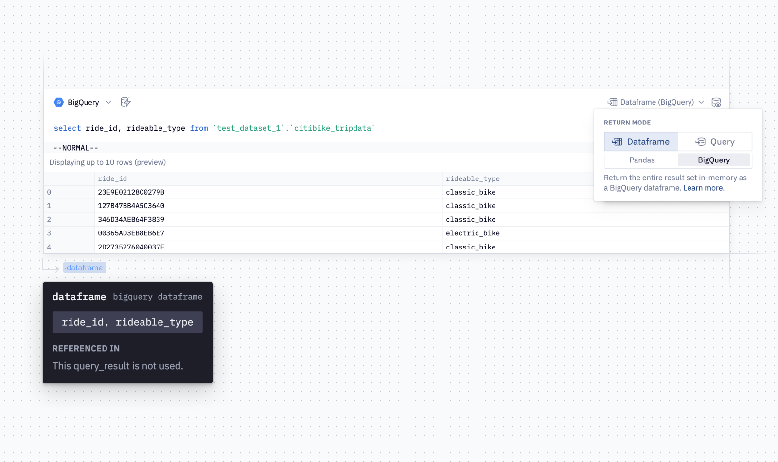
Trends in the data space such as generative AI, distributed storage systems, unstructured data formats, MLOps, and the sheer size of datasets are making it necessary to expand beyond the SQL language to truly analyze and understand your data.To provide users with more flexibility of coding languages, we announced BigQuery DataFrames at Next ‘23. Currently in preview, this new open source library gives customers the productivity of Python while allowing the BigQuery engine to handle the core processing. Offloading the Python processing to the cloud enables large scale data analysis and provides seamless production deployments along the data to AI journey.BigQuery DataFrames is a unified Python API on top of BigQuery’s managed storage and BigLake tables. It lets developers discover, describe, and understand BigQuery data by providing a Python compatible interface that can automatically scale to BigQuery sized datasets. BigQuery DataFrames also makes it easy to move into a full production application by automatically creating SQL objects like BigQuery ML inference models and Remote Functions.This is all done from the new BigQuery DataFrames package which is unified with BigQuery’s user permission model, letting Python developers use their skills and knowledge directly inside BigQuery. A bigframes.DataFrame programming object can be handed off to the Vertex AI SDK and the BigQuery DataFrames Python package is integrated with Google Cloud notebook environments such as BigQuery Studio and Colab Enterprise, as well as partner solutions like Hex, and Deepnote. It can also be installed into any Python environment with a simple ‘pip install BigQuery DataFrames’ command.Since the large-scale processing happens on the Google Cloud side, a small laptop is enough to get started. BigQuery DataFrames contains two APIs for working with BigQuery — bigframes.pandas and bigframes.ml. In this blog post, we will look at what can be done with these two APIs.bigframes.pandasLoosely based on the open source pandas API, the bigframes.pandas API is primarily designed for exploratory data analysis, advanced data manipulation, and data preparation.The BigQuery DataFrames version of the pandas API provides programming abstractions such as DataFrames and Series that pandas users are familiar with. Additionally, it comes with some distinctions that makes it easier when working with large datasets. The core capabilities of bigframes.pandas today are:Unified data Input/Output (IO): One of the primary challenges data scientists face is the fragmentation of data across various sources. BigQuery DataFrames addresses this challenge head-on with robust IO methods. Irrespective of whether the data is stored in local files, S3, GCS, or others, it can be seamlessly accessed and incorporated into BigQuery DataFrames. This interoperability not only facilitates ease of access but also effectively breaks down data silos, enabling cohesive data analysis by making disparate data sources interactable within a unified platform.code_block<ListValue: [StructValue([(‘code’, ‘# Connect a BQ table to a BigQuery table and provide a unique column for #the DatFrame index to keep the data in place on BigQueryrnbq_df = bf.read_gbq(“table”,index=[“unique_column”])rnrnrn# Read a local csv filernlocal_df = bf.read_csv(“my_data.csv”)’), (‘language’, ”), (‘caption’, <wagtail.rich_text.RichText object at 0x3efad2de9ac0>)])]>Data manipulation: Traditional workflows often involve using SQL to preprocess large datasets to a manageable size for pandas, at times losing critical data nuances. BigQuery DataFrames fundamentally alters this dynamic. With access to over 200 pandas functions, data scientists can now engage in complex operations, like handling multi-level indexes and ordering, directly within BigQuery using Python.code_block<ListValue: [StructValue([(‘code’, ‘#Obtain and prepare the datarnbq_df = bf.read_gbq(“bigquery-public-data.ml_datasets.penguins”)rnrnrn# filter down to the data we want to analyzernadelie_data = bq_df[bq_df.species == “Adelie Penguin (Pygoscelis adeliae)”]rnrnrn# drop the columns we don’t care aboutrnadelie_data = adelie_data.drop(columns=[“species”])rnrnrn# drop rows with nulls to get our training datarntraining_data = adelie_data.dropna()rnrnrn# take a peek at the training datarntraining_data.head()’), (‘language’, ”), (‘caption’, <wagtail.rich_text.RichText object at 0x3efad2de94f0>)])]>Seamless transitions back to pandas: A developer can use bigframes.pandas for large scale processing and getting to the set of data that they want to work with and then move back to traditional pandas for refined analyses on processed datasets. BigQuery DataFrames allows for a smooth transition back to traditional pandas DataFrames. Whether for advanced statistical methodologies, ML techniques, or data visualization, this interchangeability with pandas ensures that data scientists can operate within an environment they are familiar with.code_block<ListValue: [StructValue([(‘code’, ‘pandas_df = bq_df.to_pandas()’), (‘language’, ”), (‘caption’, <wagtail.rich_text.RichText object at 0x3efad2de9be0>)])]>bigframes.mlLarge-scale ML training: The ML API enhances BigQuery’s ML capabilities by introducing a Python-accessible version of BigQuery ML. It streamlines large-scale generative AI projects, offering an accessible interface reminiscent of scikit-learn. Notably, BigQuery DataFrames also integrates the latest foundation models from Vertex AI. To learn more, check out this blog on applying generative AI with BigQuery DataFrames.code_block<ListValue: [StructValue([(‘code’, ‘#Train and evaluate a linear regression model using the ML APIrnrnrnfrom bigframes.ml.linear_model import LinearRegressionrnfrom bigframes.ml.pipeline import Pipelinernfrom bigframes.ml.compose import ColumnTransformerrnfrom bigframes.ml.preprocessing import StandardScaler, OneHotEncoderrnrnrnpreprocessing = ColumnTransformer([rn(“onehot”, OneHotEncoder(), [“island”, “species”, “sex”]),rn(“scaler”, StandardScaler(), [“culmen_depth_mm”, “culmen_length_mm”, “flipper_length_mm”]),rn])rnrnrnmodel = LinearRegression(fit_intercept=False)rnrnrnpipeline = Pipeline([rn(‘preproc’, preprocessing),rn(‘linreg’, model)rn])rnrnrn# view the pipelinernpipeline’), (‘language’, ”), (‘caption’, <wagtail.rich_text.RichText object at 0x3efad2de9190>)])]>Scalable Python functions: You can also bring your ML algorithms, business logic, and libraries by deploying remote functions from BigQuery DataFrames. Creating user-developed Python functions at scale has often been a bottleneck in data science workflows. BigQuery DataFrames addresses this with a simple decorator, enabling data scientists to run scalar Python functions at BigQuery’s scale.code_block<ListValue: [StructValue([(‘code’, ‘@pd.remote_function([int], int, bigquery_connection=bq_connection_name)rndef nth_prime(n):rn prime_numbers = [2,3]rn i=3rn if(0<n<=2):rn return prime_numbers[n-1]rn elif(n>2):rn while (True):rn i+=1rn status = Truern for j in range(2,int(i/2)+1):rn if(i%j==0):rn status = Falsern breakrn if(status==True):rn prime_numbers.append(i)rn if(len(prime_numbers)==n):rn breakrn return prime_numbers[n-1]rn else:rn return -1′), (‘language’, ”), (‘caption’, <wagtail.rich_text.RichText object at 0x3efad2de9130>)])]>A full sample provided here.Vertex AI integration: Additionally, BigQuery DataFrames can provide a handoff to Vertex AI SDK for advanced modeling. The latest version of the Vertex AI SDK can directly take a bigframes.DataFrame as input without the developer having to worry about how to move or distribute the data.code_block<ListValue: [StructValue([(‘code’, ‘import vertexairnimport train_test_split as bf_train_test_splitrnrnfrom bigframes.ml.model_selection rnfrom sklearn.linear_model import LogisticRegressionrnrnspecies_categories = {rn ‘versicolor': 0,rn ‘virginica': 1,rn ‘setosa': 2,rn}rndf[‘species’] = df[‘species’].map(species_categories)rnrn# Assign an index column namernindex_col = “index”rndf.index.name = index_colrnrnfeature_columns = df[[‘sepal_length’, ‘sepal_width’, ‘petal_length’, ‘petal_width’]]rnlabel_columns = df[[‘species’]]rnbf_train_X, bf_test_X, bf_train_y, bf_test_y = bf_train_test_split(feature_columns, rn label_columns, test_size=0.2)rnrn# Enable remote mode for remote trainingrnvertexai.preview.init(remote=True)rnrn# Wrap classes to enable Vertex remote executionrnLogisticRegression = vertexai.preview.remote(LogisticRegression)rnrn# Instantiate modelrnmodel = LogisticRegression(warm_start=True)rnrn# Train model on Vertex using BigQuery DataFramesrnmodel.fit(bf_train_X, bf_train_Y)’), (‘language’, ”), (‘caption’, <wagtail.rich_text.RichText object at 0x3efad2de90d0>)])]>Hex integrationHex’s polyglot support (SQL + Python) provides BigQuery with more ways to work with BigQuery data. Users can authenticate to their BigQuery instance and seamlessly transition between SQL & Python.Hex is thrilled to be partnering with Google Cloud on their new BigQuery DataFrames functionality! The new support will unlock the ability for our customers to push computations down into their BigQuery warehouse, bypassing usual memory limits in traditional notebooks. Ariel Harnik, Head of Partnerships, HexDeepnote integrationWhen connected to a Deepnote notebook, you can read, update or delete any data directly with BigQuery SQL queries. The query result can be saved as a dataframe and later analyzed or transformed in Python, or plotted with Deepnote’s visualization cells without writing any code. Learn more about Deepnote’s integration with BigQuery.“Analyzing data and performing machine learning tasks has never been easier thanks to BigQuery’s new DataFrames. Deepnote customers are able to comfortably access the new Pandas-like API for running analytics with BigQuery DataFrames without having to worry about dataset size.” —Jakub Jurovych, CEO, DeepnoteGetting startedWatch this breakout session from Google Cloud Next ‘23 to learn more and see a demo of BigQuery DataFrames. You can get started by using the BigQuery DataFrames quickstart and sample notebooks.
Quelle: Google Cloud Platform
This post was written in collaboration with Marcelo Ochoa, the author of the Jupyter Notebook Docker Extension.
JupyterLab is a web-based interactive development environment (IDE) that allows users to create and share documents that contain live code, equations, visualizations, and narrative text. It is the latest evolution of the popular Jupyter Notebook and offers several advantages over its predecessor, including:
A more flexible and extensible user interface: JupyterLab allows users to configure and arrange their workspace to best suit their needs. It also supports a growing ecosystem of extensions that can be used to add new features and functionality.
Support for multiple programming languages: JupyterLab is not just for Python anymore! It can now be used to run code in various programming languages, including R, Julia, and JavaScript.
A more powerful editor: JupyterLab’s built-in editor includes features such as code completion, syntax highlighting, and debugging, which make it easier to write and edit code.
Support for collaboration: JupyterLab makes collaborating with others on projects easy. Documents can be shared and edited in real-time, and users can chat with each other while they work.
This article provides an overview of the JupyterLab architecture and shows how to get started using JupyterLab as a Docker extension.
Uses for JupyterLab
JupyterLab is used by a wide range of people, including data scientists, scientific computing researchers, computational journalists, and machine learning engineers. It is a powerful interactive computing and data science tool and is becoming increasingly popular as an IDE.
Here are specific examples of how JupyterLab can be used:
Data science: JupyterLab can explore data, build and train machine learning models, and create visualizations.
Scientific computing: JupyterLab can perform numerical simulations, solve differential equations, and analyze data.
Computational journalism: JupyterLab can scrape data from the web, clean and prepare data for analysis, and create interactive data visualizations.
Machine learning: JupyterLab can develop and train machine learning models, evaluate model performance, and deploy models to production.
JupyterLab can help solve problems in the following ways:
JupyterLab provides a unified environment for developing and running code, exploring data, and creating visualizations. This can save users time and effort; they do not have to switch between different tools for different tasks.
JupyterLab makes it easy to share and collaborate on projects. Documents can be shared and edited in real-time, and users can chat with each other while they work. This can be helpful for teams working on complex projects.
JupyterLab is extensible. This means users can add new features and functionality to the environment using extensions, making JupyterLab a flexible tool that can be used for a wide range of tasks.
Project Jupyter’s tools are available for installation via the Python Package Index, the leading repository of software created for the Python programming language, but you can also get the JupyterLab environment up and running using Docker Desktop on Linux, Mac, or Windows.
Figure 1: JupyterLab is a powerful web-based IDE for data science
Architecture of JupyterLab
JupyterLab follows a client-server architecture (Figure 2) where the client, implemented in TypeScript and React, operates within the user’s web browser. It leverages the Webpack module bundler to package its code into a single JavaScript file and communicates with the server via WebSockets. On the other hand, the server is a Python application that utilizes the Tornado web framework to serve the client and manage various functionalities, including kernels, file management, authentication, and authorization. Kernels, responsible for executing code entered in the JupyterLab client, can be written in any programming language, although Python is commonly used.
The client and server exchange data and commands through the WebSockets protocol. The client sends requests to the server, such as code execution or notebook loading, while the server responds to these requests and returns data to the client.
Kernels are distinct processes managed by the JupyterLab server, allowing them to execute code and send results — including text, images, and plots — to the client. Moreover, JupyterLab’s flexibility and extensibility are evident through its support for extensions, enabling users to introduce new features and functionalities, such as custom kernels, file viewers, and editor plugins, to enhance their JupyterLab experience.
Figure 2: JupyterLab architecture.
JupyterLab is highly extensible. Extensions can be used to add new features and functionality to the client and server. For example, extensions can be used to add new kernels, new file viewers, and new editor plugins.
Examples of JupyterLab extensions include:
The ipywidgets extension adds support for interactive widgets to JupyterLab notebooks.
The nbextensions package provides a collection of extensions for the JupyterLab notebook.
The jupyterlab-server package provides extensions for the JupyterLab server.
JupyterLab’s extensible architecture makes it a powerful tool that can be used to create custom development environments tailored to users’ specific needs.
Why run JupyterLab as a Docker extension?
Running JupyterLab as a Docker extension offers a streamlined experience to users already familiar with Docker Desktop, simplifying the deployment and management of the JupyterLab notebook.
Docker provides an ideal environment to bundle, ship, and run JupyterLab in a lightweight, isolated setup. This encapsulation promotes consistent performance across different systems and simplifies the setup process.
Moreover, Docker Desktop is the only prerequisite to running JupyterLabs as an extension. Once you have Docker installed, you can easily set up and start using JupyterLab, eliminating the need for additional software installations or complex configuration steps.
Getting started
Getting started with the Docker Desktop Extension is a straightforward process that allows developers to leverage the benefits of unified development. The extension can easily be integrated into existing workflows, offering a familiar interface within Docker. This seamless integration streamlines the setup process, allowing developers to dive into their projects without extensive configuration.
The following key components are essential to completing this walkthrough:
Docker Desktop
Working with JupyterLabs as a Docker extension begins with opening the Docker Desktop. Here are the steps to follow (Figure 3):
Choose Extensions in the left sidebar.
Switch to the Browse tab.
In the Categories drop-down, select Utility Tools.
Find Jupyter Notebook and then select Install.
Figure 3: Installing JupyterLab with the Docker Desktop.
A JupyterLab welcome page will be shown (Figure 4).
Figure 4: JupyterLab welcome page.
Adding extra kernels
If you need to work with other languages rather than Python3 (default), you can complete a post-installation step. For example, to add the iJava kernel, launch a terminal and execute the following:
~ % docker exec -ti –user root jupyter_embedded_dd_vm /bin/sh -c "curl -s https://raw.githubusercontent.com/marcelo-ochoa/jupyter-docker-extension/main/addJava.sh | bash"
Figure 5 shows the install process output of the iJava kernel package.
Figure 5: Capture of iJava kernel installation process.
Next, close your extension tab or Docker Desktop, then reopen, and the new kernel and language support will be enabled (Figure 6).
Figure 6: New kernel and language support enabled.
Getting started with JupyterLab
You can begin using JupyterLab notebooks in many ways; for example, you can choose the language at the welcome page and start testing your code. Or, you can upload a file to the extension using the up arrow icon found at the upper left (Figure 7).
Figure 7: Sample JupyterLab iPython notebook.
Import a new notebook from local storage (Figures 8 and 9).
Figure 8: Upload dialog from disk.
Figure 9: Uploaded notebook.
Loading JupyterLab notebook from URL
If you want to import a notebook directly from the internet, you can use the File > Open URL option (Figure 10). This page shows an example for the notebook with Java samples.
Figure 10: Load notebook from URL.
A notebook upload from URL result is shown in Figure 11.
Figure 11: Uploaded notebook from URL.
Download a notebook to your personal folder
Just like uploading a notebook, the download operation is straightforward. Select your file name and choose the Download option (Figure 12).
Figure 12: Download to local disk option menu.
A download destination option is also shown (Figure 13).
Figure 13: Select local directory for downloading destination.
A note about persistent storage
The JupyterLab extension has a persistent volume for the /home/jovyan directory, which is the default directory of the JupyterLab environment. The contents of this directory will survive extension shutdown, Docker Desktop restart, and JupyterLab Extension upgrade. However, if you uninstall the extension, all this content will be discarded. Back up important data first.
Change the core image
This Docker extension uses a Docker image — jupyter/scipy-notebook:lab-4.0.6 (ubuntu 22.04) — but you can choose one of the following available versions (Figure 14).
Figure 14: JupyterLab core image options.
To change the extension image, you can follow these steps:
Uninstall the extension.
Install again, but do not open until the next step is done.
Edit the associated docker-compose.yml file of the extension. For example, on macOS, the file can be found at: Library/Containers/com.docker.docker/Data/extensions/mochoa_jupyter-docker-extension/vm/docker-compose.yml
Change the image name from jupyter/scipy-notebook:ubuntu-22.04 to jupyter/r-notebook:ubuntu-22.04.
Open the extension.
On Linux, the docker-compose.yml file can be found at: .docker/desktop/extensions/mochoa_jupyter-docker-extension/vm/docker-compose.yml
Using JupyterLab with other extensions
To use the JupyterLab extension to interact with other extensions, such as the MemGraph database (Figure 15), typical examples only require a minimal change of the host connection option. This usually means a sample notebook referrer to MemGraph host running on localhost. Because JupyterLab is another extension hosted in a different Docker stack, you have to replace localhost with host.docker.internal, which refers to the external IP of another extension. Here is an example:
URI = "bolt://localhost:7687"
needs to be replaced by:
URI = "bolt://host.docker.internal:7687"
Figure 15: Running notebook connecting to MemGraph extension.
Conclusion
The JupyterLab Docker extension is a ready-to-run Docker stack containing Jupyter applications and interactive computing tools using a personal Jupyter server with the JupyterLab frontend.
Through the integration of Docker, setting up and using JupyterLab is remarkably straightforward, further expanding its appeal to experienced and novice users alike.
The following video provides a good introduction with a complete walk-through of JupyterLab notebooks.
Learn more
Get the latest release of Docker Desktop.
Vote on what’s next! Check out our public roadmap.
Have questions? The Docker community is here to help.
New to Docker? Get started.
Quelle: https://blog.docker.com/feed/

O2 Telefónica wird für die Vernetzung hessischer Verwaltungsbehörden ein SD-WAN errichten. Dafür hat der Mobilfunkbetreiber einen Vertrag mit dem öffentlichen IT-Dienstleister ekom21 unterzeichnet. (Telefónica, Wirtschaft)
Quelle: Golem

Die neuen Pixel-8-Geräte sollten ursprünglich offenbar 8K-Videoaufnahmen und einen Desktopmodus bekommen. (Pixel 8, Smartphone)
Quelle: Golem