This post was contributed by Thierry Moreau, co-founder and head of DevRel at OctoAI.
Generative AI models have shown immense potential over the past year with breakthrough models like GPT3.5, DALL-E, and more. In particular, open source foundational models have gained traction among developers and enterprise users who appreciate how customizable, cost-effective, and transparent these models are compared to closed-source alternatives.
In this article, we’ll explore how you can compose an open source foundational model into a streamlined image transformation pipeline that lets you manipulate images with nothing but text to achieve surprisingly good results.
With this approach, you can create fun versions of corporate logos, bring your kids’ drawings to life, enrich your product photography, or even remodel your living room (Figure 1).
Figure 1: Examples of image transformation including, from left to right: Generating creative corporate logo, bringing children’s drawings to life, enriching commercial photography, remodeling your living room
Pretty cool, right? Behind the scenes, a lot needs to happen, and we’ll walk step by step through how to reproduce these results yourself. We call the multimodal GenAI pipeline OctoShop as a nod to the popular image editing software.
Feeling inspired to string together some foundational GenAI models? Let’s dive into the technology that makes this possible.
Architecture overview
Let’s look more closely at the open source foundational GenAI models that compose the multimodal pipeline we’re about to build.
Going forward, we’ll use the term “model cocktail” instead of “multimodal GenAI model pipeline,” as it flows a bit better (and sounds tastier, too). A model cocktail is a mix of GenAI models that can process and generate data across multiple modalities: text and images are examples of data modalities across which GenAI models consume and produce data, but the concept can also extend to audio and video (Figure 2).
To build on the analogy of crafting a cocktail (or mocktail, if you prefer), you’ll need to mix ingredients, which, when assembled, are greater than the sum of their individual parts.
Figure 2: The multimodal GenAI workflow — by taking an image and text, this pipeline transforms the input image according to the text prompt.
Let’s use a Negroni, for example — my favorite cocktail. It’s easy to prepare; you need equal parts of gin, vermouth, and Campari. Similarly, our OctoShop model cocktail will use three ingredients: an equal mix of image-generation (SDXL), text-generation (Mistral-7B), and a custom image-to-text generation (CLIP Interrogator) model.
The process is as follows:
CLIP Interrogator takes in an image and generates a textual description (e.g., “a whale with a container on its back”).
An LLM model, Mistral-7B, will generate a richer textual description based on a user prompt (e.g., “set the image into space”). The LLM will consequently transform the description into a richer one that meets the user prompt (e.g., “in the vast expanse of space, a majestic whale carries a container on its back”).
Finally, an SDXL model will be used to generate a final AI-generated image based on the textual description transformed by the LLM model. We also take advantage of SDXL styles and a ControlNet to better control the output of the image in terms of style and framing/perspective.
Prerequisites
Let’s go over the prerequisites for crafting our cocktail.
Here’s what you’ll need:
Sign up for an OctoAI account to use OctoAI’s image generation (SDXL), text generation (Mistral-7B), and compute solutions (CLIP Interrogator) — OctoAI serves as the bar from which to get all of the ingredients you’ll need to craft your model cocktail. If you’re already using a different compute service, feel free to bring that instead.
Run a Jupyter notebook to craft the right mix of GenAI models. This is your place for experimenting and mixing, so this will be your cocktail shaker. To make it easy to run and distribute the notebook, we’ll use Google Colab.
Finally, we’ll deploy our model cocktail as a Streamlit app. Think of building your app and embellishing the frontend as the presentation of your cocktail (e.g., glass, ice, and choice of garnish) to enhance your senses.
Getting started with OctoAI
Head to octoai.cloud and create an account if you haven’t done so already. You’ll receive $10 in credits upon signing up for the first time, which should be sufficient for you to experiment with your own workflow here.
Follow the instructions on the Getting Started page to obtain an OctoAI API token — this will help you get authenticated whenever you use the OctoAI APIs.
Notebook walkthrough
We’ve built a Jupyter notebook in Colab to help you learn how to use the different models that will constitute your model cocktail. Here are the steps to follow:
1. Launch the notebook
Get started by launching the following Colab notebook.
There’s no need to change the runtime type or rely on a GPU or TPU accelerator — all we need is a CPU here, given that all of the AI heavy-lifting is done on OctoAI endpoints.
2. OctoAI SDK setup
Let’s get started by installing the OctoAI SDK. You’ll use the SDK to invoke the different open source foundational models we’re using, like SDXL and Mistral-7B. You can install through pip:
# Install the OctoAI SDK
!pip install octoai-sdk
In some cases, you may get a message about pip packages being previously imported in the runtime, causing an error. If that’s the case, selecting the Restart Session button at the bottom should take care of the package versioning issues. After this, you should be able to re-run the cell that pip-installs the OctoAI SDK without any issues.
3. Generate images with SDXL
You’ll first learn to generate an image with SDXL using the Image Generation solution API. To learn more about what each parameter does in the code below, check out OctoAI’s ImageGenerator client.
In particular, the ImageGenerator API takes several arguments to generate an image:
Engine: Lets you choose between versions of Stable Diffusion models, such as SDXL, SD1.5, and SSD.
Prompt: Describes the image you want to generate.
Negative prompt: Describes the traits you want to avoid in the final image.
Width, height: The resolution of the output image.
Num images: The number of images to generate at once.
Sampler: Determines the sampling method used to denoise your image. If you’re not familiar with this process, this article provides a comprehensive overview.
Number of steps: Number of denoising steps — the more steps, the higher the quality, but generally going past 30 will lead to diminishing returns.
Cfg scale: How closely to adhere to the image description — generally stays around 7-12.
Use refiner: Whether to apply the SDXL refiner model, which improves the output quality of the image.
Seed: A parameter that lets you control the reproducibility of image generation (set to a positive value to always get the same image given stable input parameters).
Note that tweaking the image generation parameters — like number of steps, number of images, sampler used, etc. — affects the amount of GPU compute needed to generate an image. Increasing GPU cycles will affect the pricing of generating the image.
Here’s an example using simple parameters:
# To use OctoAI, we'll need to set up OctoAI to use it
from octoai.clients.image_gen import Engine, ImageGenerator
# Now let's use the OctoAI Image Generation API to generate
# an image of a whale with a container on its back to recreate
# the moby logo
image_gen = ImageGenerator(token=OCTOAI_API_TOKEN)
image_gen_response = image_gen.generate(
engine=Engine.SDXL,
prompt="a whale with a container on its back",
negative_prompt="blurry photo, distortion, low-res, poor quality",
width=1024,
height=1024,
num_images=1,
sampler="DPM_PLUS_PLUS_2M_KARRAS",
steps=20,
cfg_scale=7.5,
use_refiner=True,
seed=1
)
images = image_gen_response.images
# Display generated image from OctoAI
for i, image in enumerate(images):
pil_image = image.to_pil()
display(pil_image)
Feel free to experiment with the parameters to see what happens to the resulting image. In this case, I’ve put in a simple prompt meant to describe the Docker logo: “a whale with a container on its back.” I also added standard negative prompts to help generate the style of image I’m looking for. Figure 3 shows the output:
Figure 3: An SDXL-generated image of a whale with a container on its back.
4. Control your image output with ControlNet
One thing you may want to do with SDXL is control the composition of your AI-generated image. For example, you can specify a specific human pose or control the composition and perspective of a given photograph, etc.
For our experiment using Moby (the Docker mascot), we’d like to get an AI-generated image that can be easily superimposed onto the original logo — same shape of whale and container, orientation of the subject, size, and so forth.
This is where ControlNet can come in handy: they let you constrain the generation of images by feeding a control image as input. In our example we’ll feed the image of the Moby logo as our control input.
By tweaking the following parameters used by the ImageGenerator API, we are constraining the SDXL image generation with a control image of Moby. That control image will be converted into a depth map using a depth estimation model, then fed into the ControlNet, which will constrain SDXL image generation.
# Set the engine to controlnet SDXL
engine="controlnet-sdxl",
# Select depth controlnet which uses a depth map to apply
# constraints to SDXL
controlnet="depth_sdxl",
# Set the conditioning scale anywhere between 0 and 1, try different
# values to see what they do!
controlnet_conditioning_scale=0.3,
# Pass in the base64 encoded string of the moby logo image
controlnet_image=image_to_base64(moby_image),
Now the result looks like it matches the Moby outline a lot more closely (Figure 4). This is the power of ControlNet. You can adjust the strength by varying the controlnet_conditioning_scale parameter. This way, you can make the output image more or less faithfully match the control image of Moby.
Figure 4: Left: The Moby logo is used as a control image to a ControlNet. Right: the SDXL-generated image resembles the control image more closely than in the previous example.
5. Control your image output with SDXL style presets
Let’s add a layer of customization with SDXL styles. We’ll use the 3D Model style preset (Figure 5). Behind the scenes, these style presets are adding additional keywords to the positive and negative prompts that the SDXL model ingests.
Figure 5: You can try various styles on the OctoAI Image Generation solution UI — there are more than 100 to choose from, each delivering a unique feel and aesthetic.
Figure 6 shows how setting this one parameter in the ImageGenerator API transforms our AI-generated image of Moby. Go ahead and try out more styles; we’ve generated a gallery for you to get inspiration from.
Figure 6: SDXL-generated image of Moby with the “3D Model” style preset applied.
6. Manipulate images with Mistral-7B LLM
So far we’ve relied on SDXL, which does text-to-image generation. We’ve added ControlNet in the mix to apply a control image as a compositional constraint.
Next, we’re going to layer an LLM into the mix to transform our original image prompt into a creative and rich textual description based on a “transformation prompt.”
Basically, we’re going to use an LLM to make our prompt better automatically. This will allow us to perform image manipulation using text in our OctoShop model cocktail pipeline:
Take a logo of Moby: Set it into an ultra-realistic photo in space.
Take a child’s drawing: Bring it to life in a fantasy world.
Take a photo of a cocktail: Set it on a beach in Italy.
Take a photo of a living room: Transform it into a staged living room in a designer house.
To achieve this text-to-text transformation, we will use the LLM user prompt as follows. This sets the original textual description of Moby into a new setting: the vast expanse of space.
'''
Human: set the image description into space: “a whale with a container on its back”
AI: '''
We’ve configured the LLM system prompt so that LLM responses are concise and at most one sentence long. We could make them longer, but be aware that the prompt consumed by SDXL has a 77-token context limit.
You can read more on the text generation Python SDK and its Chat Completions API used to generate text:
Model: Lets you choose out of selection of foundational open source models like Mixtral, Mistral, Llama2, Code Llama (the selection will grow with more open source models being released).
Messages: Contains a list of messages (system and user) to use as context for the completion.
Max tokens: Enforces a hard limit on output tokens (this could cut a completion response in the middle of a sentence).
Temperature: Lets you control the creativity of your answer: with a higher temperature, less likely tokens can be selected.
The choice of model, input, and output tokens will influence pricing on OctoAI. In this example, we’re using the Mistral-7B LLM, which is a great open source LLM model that really packs a punch given its small parameter size.
Let’s look at the code used to invoke our Mistral-7B LLM:
# Let's go ahead and start with the original prompt that we used in our
# image generation examples.
image_desc = "a whale with a container on its back"
# Let's then prepare our LLM prompt to manipulate our image
llm_prompt = '''
Human: set the image description into space: {}
AI: '''.format(image_desc)
# Now let's use an LLM to transform this craft clay rendition
# of Moby into a fun scify universe
from octoai.client import Client
client = Client(OCTOAI_API_TOKEN)
completion = client.chat.completions.create(
messages=[
{
"role": "system",
"content": "You are a helpful assistant. Keep your responses short and limited to one sentence."
},
{
"role": "user",
"content": llm_prompt
}
],
model="mistral-7b-instruct-fp16",
max_tokens=128,
temperature=0.01
)
# Print the message we get back from the LLM
llm_image_desc = completion.choices[0].message.content
print(llm_image_desc)
Here’s the output:
Our LLM has created a short yet imaginative description of Moby traveling through space. Figure 7 shows the result when we feed this LLM-generated textual description into SDXL.
Figure 7: SDXL-generated image of Moby where we used an LLM to set the scene in space and enrich the text prompt.
This image is great. We can feel the immensity of space. With the power of LLMs and the flexibility of SDXL, we can take image creation and manipulation to new heights. And the great thing is, all we need to manipulate those images is text; the GenAI models do the rest of the work.
7. Automate the workflow with AI-based image labeling
So far in our image transformation pipeline, we’ve had to manually label the input image to our OctoShop model cocktail. Instead of just passing in the image of Moby, we had to provide a textual description of that image.
Thankfully, we can rely on a GenAI model to perform text labeling tasks: CLIP Interrogator. Think of this task as the reverse of what SDXL does: It takes in an image and produces text as the output.
To get started, we’ll need a CLIP Interrogator model running behind an endpoint somewhere. There are two ways to get a CLIP Interrogator model endpoint on OctoAI. If you’re just getting started, we recommend the simple approach, and if you feel inspired to customize your model endpoint, you can use the more advanced approach. For instance, you may be interested in trying out the more recent version of CLIP Interrogator.
You can now invoke the CLIP Interrogator model in a few lines of code. We’ll use the fast interrogator mode here to get a label generated as quickly as possible.
# Let's go ahead and invoke the CLIP interrogator model
# Note that under a cold start scenario, you may need to wait a minute or two
# to get the result of this inference… Be patient!
output = client.infer(
endpoint_url=CLIP_ENDPOINT_URL+'/predict',
inputs={
"image": image_to_base64(moby_image),
"mode": "fast"
}
)
# All labels
clip_labels = output["completion"]["labels"]
print(clip_labels)
# Let's get just the top label
top_label = clip_labels.split(',')[0]
print(top_label)
The top label described our Moby logo as:
That’s pretty on point. Now that we’ve tested all ingredients individually, let’s assemble our model cocktail and test it on interesting use cases.
8. Assembling the model cocktail
Now that we have tested our three models (CLIP interrogator, Mistral-7B, SDXL), we can package them into one convenient function, which takes the following inputs:
An input image that will be used to control the output image and also be automatically labeled by our CLIP interrogator model.
A transformation string that describes the transformation we want to apply to the input image (e.g., “set the image description in space”).
A style string which lets us better control the artistic output of the image independently of the transformation we apply to it (e.g., painterly style vs. cinematic).
The function below is a rehash of all of the code we’ve introduced above, packed into one function.
def genai_transform(image: Image, transformation: str, style: str) -> Image:
# Step 1: CLIP captioning
output = client.infer(
endpoint_url=CLIP_ENDPOINT_URL+'/predict',
inputs={
"image": image_to_base64(image),
"mode": "fast"
}
)
clip_labels = output["completion"]["labels"]
top_label = clip_labels.split(',')[0]
# Step 2: LLM transformation
llm_prompt = '''
Human: {}: {}
AI: '''.format(transformation, top_label)
completion = client.chat.completions.create(
messages=[
{
"role": "system",
"content": "You are a helpful assistant. Keep your responses short and limited to one sentence."
},
{
"role": "user",
"content": llm_prompt
}
],
model="mistral-7b-instruct-fp16",
max_tokens=128,
presence_penalty=0,
temperature=0.1,
top_p=0.9,
)
llm_image_desc = completion.choices[0].message.content
# Step 3: SDXL+controlnet transformation
image_gen_response = image_gen.generate(
engine="controlnet-sdxl",
controlnet="depth_sdxl",
controlnet_conditioning_scale=0.4,
controlnet_image=image_to_base64(image),
prompt=llm_image_desc,
negative_prompt="blurry photo, distortion, low-res, poor quality",
width=1024,
height=1024,
num_images=1,
sampler="DPM_PLUS_PLUS_2M_KARRAS",
steps=20,
cfg_scale=7.5,
use_refiner=True,
seed=1,
style_preset=style
)
images = image_gen_response.images
# Display generated image from OctoAI
pil_image = images[0].to_pil()
return top_label, llm_image_desc, pil_image
Now you can try this out on several images, prompts, and styles.
Package your model cocktail into a web app
Now that you’ve mixed your unique GenAI cocktail, it’s time to pour it into a glass and garnish it, figuratively speaking. We built a simple Streamlit frontend that lets you deploy your unique OctoShop GenAI model cocktail and share the results with your friends and colleagues (Figure 8). You can check it on GitHub.
Follow the README instructions to deploy your app locally or get it hosted on Streamlit’s web hosting services.
Figure 8: The Streamlit app transforms images into realistic renderings in space — all thanks to the magic of GenAI.
We look forward to seeing what great image-processing apps you come up with. Go ahead and share your creations on OctoAI’s Discord server in the #built_with_octo channel!
If you want to learn how you can put OctoShop behind a Discord Bot or build your own model containers with Docker, we also have instructions on how to do that from an AI/ML workshop organized by OctoAI at DockerCon 2023.
About OctoAI
OctoAI provides infrastructure to run GenAI at scale, efficiently, and robustly. The model endpoints that OctoAI delivers to serve models like Mixtral, Stable Diffusion XL, etc. all rely on Docker to containerize models and make them easier to serve at scale.
If you go to octoai.cloud, you’ll find three complementary solutions that developers can build on to bring their GenAI-powered apps and pipelines into production.
Image Generation solution exposes endpoints and APIs to perform text to image, image to image tasks built around open source foundational models such as Stable Diffusion XL or SSD.
Text Generation solution exposes endpoints and APIs to perform text generation tasks built around open source foundational models, such as Mixtral/Mistral, Llama2, or CodeLlama.
Compute solution lets you deploy and manage any dockerized model container on capable OctoAI cloud endpoints to power your demanding GenAI needs. This compute service complements the image generation and text generation solutions by exposing infinite programmability and customizability for AI tasks that are not currently readily available on either the image generation or text generation solutions.
Disclaimer
OctoShop is built on the foundation of CLIP Interrogator and SDXL, and Mistral-7B and is therefore likely to carry forward the potential dangers inherent in these base models. It’s capable of generating unintended, unsuitable, offensive, and/or incorrect outputs. We therefore strongly recommend exercising caution and conducting comprehensive assessments before deploying this model into any practical applications.
This GenAI model workflow doesn’t work on people as it won’t preserve their likeness; the pipeline works best on scenes, objects, or animals. Solutions are available to address this problem, such as face mapping techniques (also known as face swapping), which we can containerize with Docker and deploy on OctoAI Compute solution, but that’s something to cover in another blog post.
Conclusion
This article covered the fundamentals of building a GenAI model cocktail by relying on a combination of text generation, image generation, and compute solutions powered by the portability and scalability enabled by Docker containerization.
If you’re interested in learning more about building these kinds of GenAI model cocktails, check out the OctoAI demo page or join OctoAI on Discord to see what people have been building.
Acknowledgements
The authors acknowledge Justin Gage for his thorough review, as well as Luis Vega, Sameer Farooqui, and Pedro Toruella for their contributions to the DockerCon AI/ML Workshop 2023, which inspired this article. The authors also thank Cia Bodin and her daughter Ada for the drawing used in this blog post.
Learn more
Watch the DockerCon 2023 Docker for ML, AI, and Data Science workshop.
Get the latest release of Docker Desktop.
Vote on what’s next! Check out our public roadmap.
Have questions? The Docker community is here to help.
New to Docker? Get started.
Quelle: https://blog.docker.com/feed/