Transform SQL into SQLX for Dataform

IntroductionDeveloping in SQL poses significant problems when compared to other languages and frameworks.  It’s not easy to reuse statements across different scripts, there’s no way to write tests to ensure data consistency, and dependency management requires external software solutions.  Developers will typically write thousands of lines of SQL to ensure data processing occurs in the correct order.  Additionally, documentation and metadata are afterthoughts because they need to be managed in an external catalog.Google Cloud offers Dataform and SQLX to solve these challenges. Dataform is a service for data analysts to test, develop, and deploy complex SQL workflows for data transformation in BigQuery. Dataform lets you manage data transformation in the Extraction, Loading, and Transformation (ELT) process for data integration. After extracting raw data from source systems and loading into BigQuery, Dataform helps you transform it into a well-defined, tested, and documented suite of data tables.SQLX is an open source extension of SQL and the primary tool used in Dataform. As it is an extension, every SQL file is also a valid SQLX file. SQLX brings additional features to SQL to make development faster, more reliable, and scalable. It includes functions including dependencies management, automated data quality testing, and data documentationTeams should quickly transform their SQL into SQLX to gain the full suite of benefits that Dataform provides.  This blog contains a high-level, introductory guide demonstrating this process.The steps in this guide use the Dataform on Google Cloud console. You can follow along or implement these steps with your own SQL scripts!Getting StartedHere is an example SQL script we will transform into SQLX. This script takes a source table containing reddit data. The script cleans, deduplicates, and inserts the data into a new table with a partition.code_block[StructValue([(u’code’, u’CREATE OR REPLACE TABLE reddit_stream.comments_partitionedrnPARTITION BYrn comment_daternASrnrnWITH t1 as (rnSELECTrn comment_id,rn subreddit,rn author,rn comment_text,rn CAST(total_words AS INT64) total_words,rn CAST(reading_ease_score AS FLOAT64) reading_ease_score,rn reading_ease,rn reading_grade_level,rn CAST(sentiment_score AS FLOAT64) sentiment_score,rn CAST(censored AS INT64) censored,rn CAST(positive AS INT64) positive,rn CAST(neutral AS INT64) neutral,rn CAST(negative AS INT64) negative,rn CAST(subjectivity_score AS FLOAT64) subjectivity_score,rn CAST(subjective AS INT64) subjective,rn url,rn DATE(comment_date) comment_date,rn CAST(comment_hour AS INT64) comment_hour,rn CAST(comment_year AS INT64) comment_year,rn CAST(comment_day AS INT64) comment_dayrnFROM reddit_stream.comments_streamrn)rnSELECT k.*rnFROM (rn SELECT ARRAY_AGG(row LIMIT 1)[OFFSET(0)] krn FROM t1 rowrn GROUP BY comment_idrn)’), (u’language’, u”), (u’caption’, <wagtail.wagtailcore.rich_text.RichText object at 0x3e4d73053f90>)])]1.  Create a new SQLX file and add your SQL In this guide we’ll title our file as comments_partitioned.sqlx.As you can see below, our dependency graph does not provide much information.2. Refactor SQL to remove DDL and use only SELECTIn SQLX, you only write SELECT statements. You specify what you want the output of the script to be in the config block, like a view or a table as well as other types available. Dataform takes care of adding CREATE OR REPLACE or INSERT boilerplate statements.3. Add a config object containing metadataThe config object will contain the output type, description, schema (dataset), tags, columns and their descriptions, and the BigQuery-related configuration. Check out the example below.code_block[StructValue([(u’code’, u’config {rn type: “table”,rn description: “cleaned comments data and partitioned by date for faster performance”,rn schema: “demo_optimized_staging”,rn tags: [“reddit”],rn columns: {rn comment_id: “unique id for each comment”,rn subreddit: “which reddit community the comment occurred”,rn author: “which reddit user commented”,rn comment_text: “the body of text for the comment”,rn total_words: “total number of words in the comment”,rn reading_ease_score: “a float value for comment readability score”,rn reading_ease: “a plain-text english categorization of readability”,rn reading_grade_level: “a plain-text english categorization of readability by school grade level”,rn sentiment_score: “float value for sentiment of comment between -1 and 1″,rn censored: “whether the comment needed to censoring by some process upstream”,rn positive: “one-hot encoding 1 or 0 for positive”,rn neutral: “one-hot encoding 1 or 0 for neutral”,rn negative: “one-hot encoding 1 or 0 for negative”,rn subjectivity_score: “float value for comment subjectivity score”,rn subjective: “one-hot encoding 1 or 0 for subjective”,rn url: “link to the comment on reddit”,rn comment_date: “date timestamp for when the comment occurred”,rn comment_hour: “integer for hour of comment post time”,rn comment_year: “integer for year of comment post time”,rn comment_month: “integer for month of comment post time”,rn comment_day: “integer for day of comment post time”rn },rn bigquery: {rn partitionBy: “comment_date”,rn labels: {rn cost_center: “123456”rn }rn }rn}’), (u’language’, u”), (u’caption’, <wagtail.wagtailcore.rich_text.RichText object at 0x3e4d58b5b190>)])]4. Create declarations for any source tablesIn our SQL script, we directly write reddit_stream.comments_stream. In SQLX, we’ll want to utilize a declaration to create relationships between source data and tables created by Dataform. Add a new comments_stream.sqlx file to your project for this declaration:code_block[StructValue([(u’code’, u’config {rn type: “declaration”,rn database: “my-project”,rn schema: “reddit_stream”,rn name: “comments_stream”,rn description: “A BigQuery table acting as a data sink for comments streaming in real-time.”rn}’), (u’language’, u”), (u’caption’, <wagtail.wagtailcore.rich_text.RichText object at 0x3e4d7271f710>)])]We’ll utilize this declaration in the next step.5. Add references to declarations, tables, and views.This will help build the dependency graph.  In our SQL script, there is a single reference to the declaration. Simply replace reddit_stream.comments_stream with ${ref(“comments_stream”)}. Managing dependencies with the ref function has numerous advantages.The dependency tree complexity is abstracted away. Developers simply need to use the ref function and list dependencies.It enables us to write smaller, more reusable and more modular queries instead of thousand-line-long queries. That makes pipelines easier to debug.You get alerted in real time about issues like missing or circular dependencies6. Add assertions for data validationYou can define data quality tests, called assertions, directly from the config block of your SQLX file. Use assertions to check for uniqueness, null values or any custom row condition. The dependency tree adds assertions for visibility.Here are assertions for our example:code_block[StructValue([(u’code’, u’assertions: {rn uniqueKey: [“comment_id”],rn nonNull: [“comment_text”],rn rowConditions: [rn “total_words > 0″rn ]rn }’), (u’language’, u”), (u’caption’, <wagtail.wagtailcore.rich_text.RichText object at 0x3e4d7271fd10>)])]These assertions will pass if comment_id is a unique key, if comment_text is non-null, and if all rows have total_words greater than zero.7. Utilize JavaScript for repeatable SQL and parameterizationOur example has a deduplication SQL block.  This is a perfect opportunity to create a JavaScript function to reference this functionality in other SQLX files.  For this scenario, we’ll create the includes folder and add a common.js file with the following contents:code_block[StructValue([(u’code’, u’function dedupe(table, group_by_cols) {rn return `rnSELECT k.*rnFROM (rn SELECT ARRAY_AGG(row LIMIT 1)[OFFSET(0)] krn FROM ${table} rowrn GROUP BY ${group_by_cols}rn)rn `rn}rnrnmodule.exports = { dedupe };’), (u’language’, u”), (u’caption’, <wagtail.wagtailcore.rich_text.RichText object at 0x3e4d7271f610>)])]Now, we can replace that code block with this function call in our SQLX file as such: ${common.dedupe(“t1″, “comment_id”)}In certain scenarios, you may want to use constants in your SQLX files. Let’s add a constants.js file to our includes folder and create a cost center dictionary.code_block[StructValue([(u’code’, u’const COST_CENTERS = {rn dev: “000000”,rn stage: “123123”,rn prod: “123456”rn}rnrnmodule.exports = { COST_CENTERS }’), (u’language’, u”), (u’caption’, <wagtail.wagtailcore.rich_text.RichText object at 0x3e4d7271f910>)])]We can use this to label our output BigQuery table with a cost center.  Here’s an example of using the constant in a SQLX config block:code_block[StructValue([(u’code’, u’bigquery: {rn partitionBy: “comment_date”,rn labels: {rn cost_center: constants.COST_CENTERS.devrn }rn }’), (u’language’, u”), (u’caption’, <wagtail.wagtailcore.rich_text.RichText object at 0x3e4d7271f990>)])]8. Validate the final SQLX file and compiled dependency graphAfter completing the above steps, let’s have a look at the final SQLX files:comments_stream.sqlxcode_block[StructValue([(u’code’, u’config {rn type: “declaration”,rn database: “my-project”,rn schema: “reddit_stream”,rn name: “comments_stream”,rn description: “A BigQuery table acting as a data sink for comments streaming in real-time.”rn}’), (u’language’, u”), (u’caption’, <wagtail.wagtailcore.rich_text.RichText object at 0x3e4d7271f750>)])]comments_partitioned.sqlxcode_block[StructValue([(u’code’, u’config {rn type: “table”,rn description: “cleaned comments data and partitioned by date for faster performance”,rn schema: “demo_optimized_staging”,rn tags: [“reddit”],rn columns: {rn comment_id: “unique id for each comment”,rn subreddit: “which reddit community the comment occurred”,rn author: “which reddit user commented”,rn comment_text: “the body of text for the comment”,rn total_words: “total number of words in the comment”,rn reading_ease_score: “a float value for comment readability score”,rn reading_ease: “a plain-text english categorization of readability”,rn reading_grade_level: “a plain-text english categorization of readability by school grade level”,rn sentiment_score: “float value for sentiment of comment between -1 and 1″,rn censored: “whether the comment needed to censoring by some process upstream”,rn positive: “one-hot encoding 1 or 0 for positive”,rn neutral: “one-hot encoding 1 or 0 for neutral”,rn negative: “one-hot encoding 1 or 0 for negative”,rn subjectivity_score: “float value for comment subjectivity score”,rn subjective: “one-hot encoding 1 or 0 for subjective”,rn url: “link to the comment on reddit”,rn comment_date: “date timestamp for when the comment occurred”,rn comment_hour: “integer for hour of comment post time”,rn comment_year: “integer for year of comment post time”,rn comment_month: “integer for month of comment post time”,rn comment_day: “integer for day of comment post time”rn },rn bigquery: {rn partitionBy: “comment_date”,rn labels: {rn cost_center: constants.COST_CENTERS.devrn }rn },rn assertions: {rn uniqueKey: [“comment_id”],rn nonNull: [“comment_text”],rn rowConditions: [rn “total_words > 0″rn ]rn }rn}rnrnWITH t1 as (rnSELECTrn comment_id,rn subreddit,rn author,rn comment_text,rn CAST(total_words AS INT64) total_words,rn CAST(reading_ease_score AS FLOAT64) reading_ease_score,rn reading_ease,rn reading_grade_level,rn CAST(sentiment_score AS FLOAT64) sentiment_score,rn CAST(censored AS INT64) censored,rn CAST(positive AS INT64) positive,rn CAST(neutral AS INT64) neutral,rn CAST(negative AS INT64) negative,rn CAST(subjectivity_score AS FLOAT64) subjectivity_score,rn CAST(subjective AS INT64) subjective,rn url,rn DATE(comment_date) comment_date,rn CAST(comment_hour AS INT64) comment_hour,rn CAST(comment_year AS INT64) comment_year,rn CAST(comment_month AS INT64) comment_month,rn CAST(comment_day AS INT64) comment_dayrnFROM ${ref(‘comments_stream’)}rnWHERE CAST(total_words AS INT64) > 0)rnrnrn${common.dedupe(“t1″, “comment_id”)}’), (u’language’, u”), (u’caption’, <wagtail.wagtailcore.rich_text.RichText object at 0x3e4d72d0e410>)])]Let’s validate the dependency graph and ensure the order of operations looks correct.Now it’s easy to visualize where the source data is coming from, what output type comments_partitioned is, and what data quality tests will occur!Next StepsThis guide outlines the first steps of transitioning legacy SQL solutions to SQLX and Dataform for improved metadata management, comprehensive data quality testing, and efficient development. Adopting Dataform streamlines the management of your cloud data warehouse processes allowing you to focus more on analytics and less on infrastructure management. For more information, check out Google Cloud’s Overview of Dataform.  Explore our official Dataform guides and Dataform sample script library for even more hands-on experiences.Related ArticleDataform is joining Google Cloud: Deploy data transformations with SQL in BigQueryWith our acquisition of Dataform, you can now leverage software development best practices to define, document, test and deploy data tran…Read Article
Quelle: Google Cloud Platform

How to migrate Cloud Storage data from multi-region to regional

There are many considerations to take into account when choosing the location type of your Cloud Storage bucket. However, as business needs change, you may find that regional storage offers lower cost and/or better performance than multi-region or dual-region storage. By design, once your data is already stored in a bucket, the location type of that bucket cannot be changed. The path forward is clear: you must create new, regional buckets and move your existing data into them.Migrating from multi-region to regional storageThe tool for this job is the Storage Transfer Service (STS), which uses parameterization to bulk migrate files. The basic steps are as follows:Create new buckets in the region you desire.Use STS to transfer the objects from the original multi-region buckets to the new regional ones.Test the objects (e.g., using Cloud Storage Insights) in the new buckets and if the test is passed, delete the old buckets.While there is no charge for use of the STS itself, performing a migration will incur Cloud Storage charges associated with the move — including storage charges for the data in the source and destination until you delete the source bucket; for the Class A and B operations involved in listing, reading, and writing the objects; for egress charges for moving the data across the network; and retrieval and/or early delete fees associated with migrating Nearline, Coldline and Archive objects. Please see the STS pricing documentation for more information.Though we have focused on a multi-region to regional Cloud Storage migration, in the steps that follow, the considerations and process for any other type of location change will be much the same — for example, you might want to migrate from multi-region to dual-region, which could be a good middle ground between the options, or even migrate a regional bucket from one location to a different regional location.Planning the migrationThe first determination will be which buckets to migrate. There could be a number of reasons why you would choose not to migrate certain buckets, for example, the data inside might be stale and/or not needed anymore, or it might serve a workload that is a better fit for multi-region, for example, an image hosting service for an international user base. If you’re transferring massive amounts of data, it is also important to consider the time it will take to complete the transfer. To prevent any one customer from overloading the service, the STS has queries per second and bandwidth limitations at a project level. If you’re planning a massive migration (say over 100PB or 1 billion objects) you should notify your Google Cloud sales team or create a support ticket to ensure that the required capacity is available in the region where you’re doing the transfer. Your sales team can also help you calculate the time the transfer will take, which is a complex process that involves many factors. To determine if you need to be worried about how long the transfer could take, consider the following data points: A bucket with 11PB of data and 70 million objects should take around 24 hours to transfer. A bucket with 11PB of data and 84 billion objects could take 3 years to transfer if jobs are not executed concurrently. In general, if the number of objects you need to transfer is over a billion, the transfer could take prohibitively long, so you will need to work with Google Cloud technicians to reduce the transfer time by parallelizing the transfer. Note that these metrics are for cloud to cloud transfers, not HTTP transfers. There may also be metadata that you want to transfer from your old buckets to your new buckets. Some metadata, like user-created custom fields, are automatically transferred by the STS, whereas other fields, like storage classes or CMEK, must be manually enabled via the STS API. The API or gcloud CLI must also be used if you wish to transfer all versions of your objects, as opposed to just the latest one. If you are using Cloud Storage Autoclass in the destination bucket (it must be enabled at bucket creation time), all of your objects will start out as a Standard storage class after the transfer. Refer to the Transfer between Cloud Storage buckets documentation for guidance on handling all complexities you may have to account for.Your final decision point will be whether you want to keep the exact same names for your buckets, or whether you can work with new bucket names (e.g., no application changes with the same bucket name). As you will see in the next section, the migration plan will require an additional step if you need to keep the original names.Steps for migrationThe diagram below shows how the migration process will unfold for a single bucket.You may decide that in order to avoid having to recode the names of the buckets in every downstream application, you want your regional buckets to have the exact same names as your original multi-region buckets did. Since bucket names are as immutable as their location types, and the names need to be globally unique, this requires transferring your data twice: once to temporary intermediate buckets, then to the new target buckets that were created after the source buckets had been deleted. While this will obviously take additional time, it should be noted that the second transfer to the new target buckets will take approximately a tenth of the time of the first transfer because you are doing a simple copy within a region.Be sure to account for the fact that there will be downtime for your services while you are switching them to the new buckets. Also keep in mind that when you delete the original multi-region buckets, you should create the regional buckets with the same name immediately afterwards. Once you’ve deleted them, theoretically anyone can claim their names. If you are aiming to transfer multiple buckets, you can run multiple jobs simultaneously to decrease the overall migration time. STS supports around 200 concurrent jobs per project. Additionally, if you have very large buckets, either by size or number of objects, it is possible that the job may take several days to fully transfer the data in the bucket, as each job will copy one object at a time. In these cases, you can run multiple jobs per bucket and configure each job to filter objects by prefix. If configured correctly, this can significantly reduce the overall migration time for very large buckets. This library can help with managing your STS jobs, and testing the objects that have been transferred.What’s next?With great flexibility of storage options comes great responsibility. To determine whether a migration is necessary, you will need to do a careful examination of your data, and the workloads that use it. You will also need to consider what data and metadata should be transferred to the buckets of the new location type. Luckily, once you’ve made the decisions, Cloud Storage and the STS make it easy to migrate your data. Once your data is transferred, there are other ways to optimize your usage of Cloud Storage, such as leveraging customizable monitoring dashboards. If you’re not using the STS, perhaps for smaller transfers or analytical workloads where you’re downloading and uploading data to a VM, consider using the gcloud storage CLI.Related ArticleBest practices for Cloud Storage cost optimizationFind tips here on optimizing your Cloud Storage buckets or objects based on your company’s performance, retention, and access pattern req…Read Article
Quelle: Google Cloud Platform

Submit your entry now for our *new* Talent Transformation Google Cloud Customer Award

Has your business made talent investments that directly link to your digital transformation strategy? Google Cloud wants to honor your organization for its dedication to developing your team’s Google Cloud skills through our *new* Talent Transformation Google Cloud Customer Award. Submit your application before March 31, 2023 to be recognized as a global leader in cloud talent transformation. Celebrating Google Cloud customer’s outstanding contributionsGoogle Cloud Customer Awards recognize organizations who are leading business transformation with Google Cloud products and solutions. We want to hear how you are growing one of the most important elements of your organization — your people! Tell us your story for a chance to win and enjoy benefits like:A Google Cloud Customer Award designation for your websiteCollaboration with Google Cloud leaders, engineers and product managers at a variety of roundtables, discussions and eventsGoogle Cloud press release and announcement support to help strengthen your brand as a visionary leader in technologyPromotion through the Google Cloud results blog and social media to share your success story with our extensive customer and partner networkInclusion in the annual Google Cloud Customer ebookA place amongst the global leaders who are recognized at Google Cloud events and celebrationsHow to get started and tips for a submission that will stand outTell your compelling and unique story about cloud talent transformation! This can include mentorship, skills training, Google Cloud certification preparation support or anything you’ve built to invest in your people’s Google Cloud skills. To help your accomplishments shine, use the distinct voice and personality of your organization. You’ll want to begin by gathering:Business and deployment metricsSolution overview diagrams, workflows, architectural diagrams or imagesExisting public case studies, webinars or other contentThese awards recognize customers who demonstrate unique transformation and innovation, business/operational excellence, industry-wide problem solving, and implementing long-term, lasting benefits. You can add depth to your submission by asking stakeholders to share their perspectives — for example, your CEO or customer testimonies are great ways to do this.Metrics and impact are also important. Share how your company is now faster, smarter, more collaborative and flexible due to the Google Cloud skills development opportunities that you provided.Judging the entries and results announcementsA diverse panel of senior technical judges from around the world carefully assess hundreds of entries that are ranked using a scoring framework. We ensure high quality assessment through a three-round process, using specified benchmarks at least twice per entry. The Google Cloud Customer Awards team and the judges are the only people who see submissions, and winners are under embargo until official announcements take place. All participants will be notified of results via email at least two months prior to announcements, with results notification scheduled for May 31, 2023.Results will be formally announced and celebrated at a special event later this year, where winners take their place amongst other outstanding leaders in innovative thinking and business transformation.For inspiration and to learn more about the transformative organizations that have won Customer Awards with their visionary achievements, take a look at last year’s industry winners. We encourage entry by any customers – new to established, small to large, across all types of products and solutions. Submitting your entryIn order to enter, you must be a Google Cloud customer, with success you can demonstrate within the last 12 months. Google Cloud partners and Googlers can also submit on behalf of customers.Award categories include Industry Customer Awards across a range of verticals, and our Technology for Good Awards, which include the Talent Transformation Award. You may apply for one Industry Customer Award, plus any or all of the Technology for Good Awards.Start by using this templateto gather all of the relevant information as a team. Designate one person to complete the application and submit via the Customer Awards online questionnaire. The submission window is now open through March 31, 2023.We are so excited to hear about the wonderful things you are doing to empower your teams to build upon their Google Cloud knowledge and skills — making you a leader in your industry. Happy submitting — get started here!
Quelle: Google Cloud Platform

How to use advance feature engineering to preprocess data in BigQuery ML

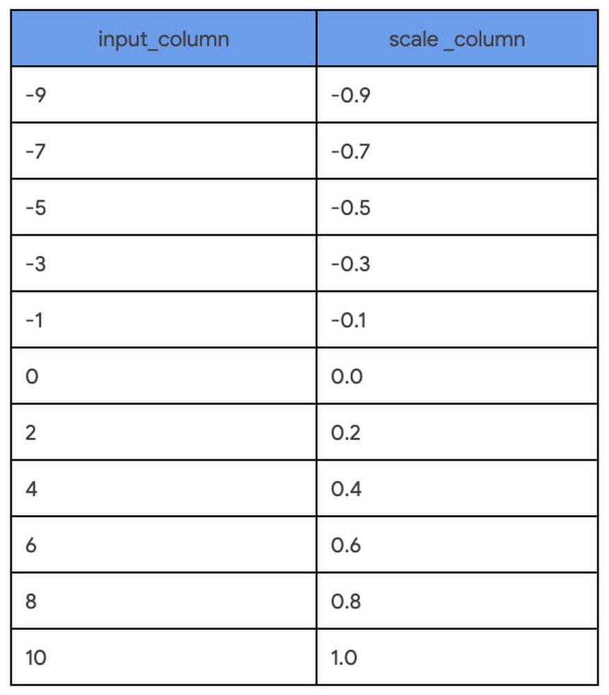
Preprocessing and transforming raw data into features is a critical but time consuming step  in the ML process.  This is especially true when a data scientist or data engineer has to move data across different platforms to do MLOps. In this blogpost, we describe how we streamline this process by adding two feature engineering capabilities in BigQuery ML.Our previous blog outlines the data to AI journey with BigQuery ML, highlighting two powerful features that simplify MLOps – data preprocessing functions for feature engineering and the ability to export BigQuery ML TRANSFORM statement as part of the model artifact. In this blog post, we share how to use these features for creating a seamless experience from BigQuery ML to Vertex AI.Data Preprocessing FunctionsPreprocessing and transforming raw data into features is a critical but time consuming step when operationalizing ML. We recently announced the public preview of advanced feature engineering functions in BigQuery ML. These functions help you impute, normalize or encode data. When this is done inside the database, BigQuery, the entire process becomes easier, faster, and more secure to preprocess data.Here is a list of the new functions we are introducing in this release. The full list of preprocessing functions can be found here.ML.MAX_ABS_SCALERScale a numerical column to the range [-1, 1] without centering by dividing by the maximum absolute value.ML.ROBUST_SCALERScale a numerical column by centering with the median (optional) and dividing by the quantile range of choice ([25, 75] by default).ML.NORMALIZERTurn an input numerical array into a unit norm array for any p-norm: 0, 1, >1, +inf. The default is 2 resulting in a normalized array where the sum of squares is 1.ML.IMPUTERReplace missing values in a numerical or categorical input with the mean, median or mode (most frequent).ML.ONE_HOT_ENCODEROne-hot encode a categorical input. Also, it optionally does dummy encoding by dropping the most frequent value. It is also possible to limit the size of the encoding by specifying k for the k most frequent categories and/or a lower threshold for the frequency of categories. ML.LABEL_ENCODEREncode a categorical input to integer values [0, n categories] where 0 represents NULL and excluded categories. You can exclude categories by specifying k for k most frequent categories and/or a lower threshold for the frequency of categories.Model Export with TRANSFORM StatementYou can now export BigQuery ML models that include a feature TRANSFORM statement. The ability to include TRANSFORM statements makes models more portable when exporting them for online prediction. This capability also works when BigQuery ML models are registered with Vertex AI Model Registry and deployed to Vertex AI Prediction endpoints. More details about exporting models can be found in BigQuery ML Exporting models.These new features are available through the Google Cloud Console, BigQuery API, and client libraries. Step-by-step guide to use the two featuresIn this tutorial, we will use the bread recipe competition dataset to predict judges rating using linear regression and boosted tree models.Objective: To demonstrate how to preprocess data using the new functions, register the model with Vertex AI Model Registry, and deploy the model for online prediction with Vertex AI Prediction endpoints. Dataset: Each row represents a bread recipe with columns for each ingredient (flour, salt, water, yeast) and procedure (mixing time, mixing speed, cooking temperature, resting time). There are also columns that include judges ratings of the final product from each recipe.Overview of the tutorial: Steps 1 and 2 show how to use the TRANSFORM statement. Steps 3 and 4 demonstrate how to manually export and register the models. Steps 5 through 7 show how to deploy a model to Vertex AI Prediction endpoint.For the best learning experience, follow this blog post alongside the tutorial notebook.Step 1: Transform BigQuery columns into ML features with SQLBefore training an ML model, exploring the data within columns is essential to identifying the data type, distribution, scale, missing patterns, and extreme values.  BigQuery ML enables this exploratory analysis with SQL. With the new preprocessing functions it is now even easier to transform BigQuery columns into ML features with SQL while iterating to find the optimal transformation. For example, when using the ML.MAX_ABS_SCALER function for an input column, each value is divided by the maximum absolute value (10 in the example): code_block[StructValue([(u’code’, u’SELECTrn input_column,rn ML.MAX_ABS_SCALER (input_column) OVER() AS scale_columnrnFROMrn UNNEST([0, -1, 2, -3, 4, -5, 6, -7, 8, -9, 10]) as input_columnrnORDER BY input_column’), (u’language’, u”), (u’caption’, <wagtail.wagtailcore.rich_text.RichText object at 0x3ea90d564c90>)])]Once the input columns for an ML model are identified and the feature transformations are chosen, it is enticing to apply the transformation and save the output as a view. But this has an impact on our predictions later on because these same transformations will need to be applied before requesting predictions. Step 2 shows how to prevent this separation of processing and model training.Step 2: Iterate through multiple models with inline TRANSFORM functionsBuilding on the preprocessing explorations in Step 1, the chosen transformations are applied inline with model training using the TRANSFORM statement. This interlocks the model iteration with the preprocessing explorations while making any candidate ready for serving with BigQuery or beyond. This means you can immediately try multiple model types without any delayed impact of feature transformations on predictions. In this step, two models, linear regression and boosted tree, are trained side-by-side with identical TRANSFORM statements:Training with linear regression – Model acode_block[StructValue([(u’code’, u”CREATE OR REPLACE MODEL `statmike-mlops-349915.feature_engineering.03_feature_engineering_2a`rnTRANSFORM (rn JUDGE_A,rnrn ML.MIN_MAX_SCALER(flourAmt) OVER() as scale_flourAmt, rn ML.ROBUST_SCALER(saltAmt) OVER() as scale_saltAmt,rn ML.MAX_ABS_SCALER(yeastAmt) OVER() as scale_yeastAmt,rn ML.STANDARD_SCALER(water1Amt) OVER() as scale_water1Amt,rn ML.STANDARD_SCALER(water2Amt) OVER() as scale_water2Amt,rnrn ML.STANDARD_SCALER(waterTemp) OVER() as scale_waterTemp,rn ML.ROBUST_SCALER(bakeTemp) OVER() as scale_bakeTemp,rn ML.MIN_MAX_SCALER(ambTemp) OVER() as scale_ambTemp,rn ML.MAX_ABS_SCALER(ambHumidity) OVER() as scale_ambHumidity,rnrn ML.ROBUST_SCALER(mix1Time) OVER() as scale_mix1Time,rn ML.ROBUST_SCALER(mix2Time) OVER() as scale_mix2Time,rn ML.ROBUST_SCALER(mix1Speed) OVER() as scale_mix1Speed,rn ML.ROBUST_SCALER(mix2Speed) OVER() as scale_mix2Speed,rn ML.STANDARD_SCALER(proveTime) OVER() as scale_proveTime,rn ML.MAX_ABS_SCALER(restTime) OVER() as scale_restTime,rn ML.MAX_ABS_SCALER(bakeTime) OVER() as scale_bakeTimern)rnOPTIONS (rn model_type = ‘LINEAR_REG’,rn input_label_cols = [‘JUDGE_A’],rn enable_global_explain = TRUE,rn data_split_method = ‘AUTO_SPLIT’,rn MODEL_REGISTRY = ‘VERTEX_AI’,rn VERTEX_AI_MODEL_ID = ‘bqml_03_feature_engineering_2a’,rn VERTEX_AI_MODEL_VERSION_ALIASES = [‘run-20230112234821′]rn ) ASrnSELECT * EXCEPT(Recipe, JUDGE_B)rnFROM `statmike-mlops-349915.feature_engineering.bread`”), (u’language’, u”), (u’caption’, <wagtail.wagtailcore.rich_text.RichText object at 0x3ea90e7bcc90>)])]Training with boosted tree – Model bcode_block[StructValue([(u’code’, u”CREATE OR REPLACE MODEL `statmike-mlops-349915.feature_engineering.03_feature_engineering_2b`rnTRANSFORM (rn JUDGE_A,rnrn ML.MIN_MAX_SCALER(flourAmt) OVER() as scale_flourAmt, rn ML.ROBUST_SCALER(saltAmt) OVER() as scale_saltAmt,rn ML.MAX_ABS_SCALER(yeastAmt) OVER() as scale_yeastAmt,rn ML.STANDARD_SCALER(water1Amt) OVER() as scale_water1Amt,rn ML.STANDARD_SCALER(water2Amt) OVER() as scale_water2Amt,rnrn ML.STANDARD_SCALER(waterTemp) OVER() as scale_waterTemp,rn ML.ROBUST_SCALER(bakeTemp) OVER() as scale_bakeTemp,rn ML.MIN_MAX_SCALER(ambTemp) OVER() as scale_ambTemp,rn ML.MAX_ABS_SCALER(ambHumidity) OVER() as scale_ambHumidity,rnrn ML.ROBUST_SCALER(mix1Time) OVER() as scale_mix1Time,rn ML.ROBUST_SCALER(mix2Time) OVER() as scale_mix2Time,rn ML.ROBUST_SCALER(mix1Speed) OVER() as scale_mix1Speed,rn ML.ROBUST_SCALER(mix2Speed) OVER() as scale_mix2Speed,rn ML.STANDARD_SCALER(proveTime) OVER() as scale_proveTime,rn ML.MAX_ABS_SCALER(restTime) OVER() as scale_restTime,rn ML.MAX_ABS_SCALER(bakeTime) OVER() as scale_bakeTimern)rnOPTIONS (rn model_type = ‘BOOSTED_TREE_REGRESSOR’,rn booster_type = ‘GBTREE’,rn num_parallel_tree = 1,rn max_iterations = 30,rn early_stop = TRUE,rn min_rel_progress = 0.01,rn tree_method = ‘HIST’,rn subsample = 0.85, rn input_label_cols = [‘JUDGE_A’],rn enable_global_explain = TRUE,rn data_split_method = ‘AUTO_SPLIT’,rn l1_reg = 10,rn l2_reg = 10,rn MODEL_REGISTRY = ‘VERTEX_AI’,rn VERTEX_AI_MODEL_ID = ‘bqml_03_feature_engineering_2b’,rn VERTEX_AI_MODEL_VERSION_ALIASES = [‘run-20230112234926′]rn ) ASrnSELECT * EXCEPT(Recipe, JUDGE_B)rnFROM `statmike-mlops-349915.feature_engineering.bread`”), (u’language’, u”), (u’caption’, <wagtail.wagtailcore.rich_text.RichText object at 0x3ea8f93a6a90>)])]Identical input columns that have the same preprocessing means you can easily compare the accuracy of the models. Using the BigQuery ML function ML.EVALUATE makes this comparison as simple as a single SQL query that stacks these outcomes with the UNION ALL set operator:code_block[StructValue([(u’code’, u”SELECT ‘Manual Feature Engineering – 2A’ as Approach, mean_squared_error, r2_scorernFROM ML.EVALUATE(MODEL `statmike-mlops-349915.feature_engineering.03_feature_engineering_2a`)rnUNION ALLrnSELECT ‘Manual Feature Engineering – 2B’ as Approach, mean_squared_error, r2_scorernFROM ML.EVALUATE(MODEL `statmike-mlops-349915.feature_engineering.03_feature_engineering_2b`)”), (u’language’, u”), (u’caption’, <wagtail.wagtailcore.rich_text.RichText object at 0x3ea90c7bd310>)])]The results of the evaluation comparison show that using the boosted tree model results in a much better model than linear regression with drastically lower mean squared error and higher r2. Both models are ready to serve predictions, but the clear choice is the boosted tree regressor. Once we decide which model to use, you can predict directly within BigQuery ML using the ML.PREDICT function. In the rest of the tutorial, we show how to export the model outside of BigQuery ML and predict using Google Cloud Vertex AI.Using BigQuery Models for Inference Outside of BigQueryOnce your model is trained, if you want to do online inference for low latency responses in your application for online prediction, you have to deploy the model outside of BigQuery. The following steps demonstrate how to deploy the models to Vertex AI Prediction endpoints.This can be accomplished in one of two ways:Manually export the model from BigQuery ML and set up a Vertex AI Prediction Endpoint. To do this, you need to do steps 3 and 4 first.Register the model and deploy from Vertex AI Model Registry automatically. The capability is not available yet but will be available in a forthcoming release. Once it’s available steps 3 and 4 can be skipped.Step 3. Manually export models from BigQueryBigQuery ML supports an EXPORT MODEL statement to deploy models outside of BigQuery. A manual export includes two models – a preprocessing model that reflects the TRANSFORM statement and a prediction model. Both models are exported with a single export statement in BigQuery ML.code_block[StructValue([(u’code’, u”EXPORT MODEL `statmike-mlops-349915.feature_engineering.03_feature_engineering_2b`rn OPTIONS (URI = ‘gs://statmike-mlops-349915-us-central1-bqml-exports/03/2b/model’)”), (u’language’, u”), (u’caption’, <wagtail.wagtailcore.rich_text.RichText object at 0x3ea8faf965d0>)])]The preprocessing model that captures the TRANSFORM statement is exported as a TensorFlow SavedModel file. In this example it is exported to a GCS bucket located at ‘gs://statmike-mlops-349915-us-central1-bqml-exports/03/2b/model/transform’.  The prediction models are saved in portable formats that match the frameworks in which they were trained by BigQuery ML. The linear regression model is exported as a TensorFlow SavedModel and the boosted tree regressor is exported as Booster file (XGBoost). In this example, the boost tree model is exported to a GCS bucket located at ‘gs://statmike-mlops-349915-us-central1-bqml-exports/03/2b/model’ These export files are in a standard open format of the native model types making them completely portable to be deployed anywhere – they can be deployed to Vertex AI (Steps 4-7 below), on your own infrastructure, or even in edge applications.Steps 4 through 7 show how to register and deploy a model to Vertex AI Prediction endpoint. These steps need to be repeated separately for the preprocessing models and the prediction models.Step 4. Register models to Vertex AI Model RegistryTo deploy the models in Vertex AI Prediction, they first need to be registered with the Vertex AI Model Registry To do this two inputs are needed – the links to the model files and a URI to a pre-built container. Go to Step 4 in the tutorial to see how exactly it’s done.The registration can be done with the Vertex AI console or programmatically with one of the clients. In the example below, the Python client for Vertex AI is used to register the models like this:code_block[StructValue([(u’code’, u’vertex_model = aiplatform.Model.upload(rn display_name = ‘gcs_03_feature_engineering_2b’,rn serving_container_image_uri = ‘us-docker.pkg.dev/vertex-ai/prediction/xgboost-cpu.1-1:latest’,rn artifact_uri = “gs://statmike-mlops-349915-us-central1-bqml-exports/03/2b/model”rn)’), (u’language’, u”), (u’caption’, <wagtail.wagtailcore.rich_text.RichText object at 0x3ea8faf96650>)])]Step 5. Create Vertex AI Prediction endpointsVertex AI includes a service forhosting models for online predictions. To host a model on a Vertex AI Prediction endpoint you first create an endpoint. This can also be done directly from the Vertex AI Model Registry console or programmatically with one of the clients. In the example below, the Python client for Vertex AI is used to create the endpoint like this:code_block[StructValue([(u’code’, u’vertex_endpoint = aiplatform.Endpoint.create (rn display_name = u201803_feature_engineering_manual_2bu2019rn)’), (u’language’, u”), (u’caption’, <wagtail.wagtailcore.rich_text.RichText object at 0x3ea8faf96b50>)])]Step 6. Deploy models to endpointsDeploying a model from the Vertex AI Model Registry (Step 4) to a Vertex AI Prediction endpoint (Step 5) is done in a single deployment action where the model definition is supplied to the endpoint along with the type of machine to utilize. Vertex AI Prediction endpoints can automatically scale up or down to handle prediction traffic needs by providing the number of replicas to utilize (default is 1 for min and max). In the example below, the Python client for Vertex AI is being used with the deploy method for the endpoint (Step 5) using the models (Step 4):code_block[StructValue([(u’code’, u”vertex_endpoint.deploy(rn model = vertex_model,rn deployed_model_display_name = vertex_model.display_name,rn traffic_percentage = 100,rn machine_type = ‘n1-standard-2′,rn min_replica_count = 1,rn max_replica_count = 1rn)”), (u’language’, u”), (u’caption’, <wagtail.wagtailcore.rich_text.RichText object at 0x3ea90c7bd450>)])]Step 7. Request predictions from endpoints  Once the model is deployed to a Vertex AI Prediction endpoint (Step 6) it can serve predictions. Rows of data, called instances, are passed to the endpoint and results are returned that include the processed information: preprocessing result or prediction. Getting prediction results from Vertex AI Prediction endpoints can be done with any of the Vertex AI API interfaces (REST, gRPC, gcloud, Python, Java, Node.js). Here, the request is demonstrated directly with the predict method of the endpoint (Step 6) using the Python client for Vertex AI as follows:code_block[StructValue([(u’code’, u”results = vertex_endpoint.predict(instances = [rn{‘flourAmt': 511.21695405324624,rn ‘saltAmt': 9,rn ‘yeastAmt': 11,rn ‘mix1Time': 6,rn ‘mix1Speed': 4,rn ‘mix2Time': 5,rn ‘mix2Speed': 4,rn ‘water1Amt': 338.3989183746999,rn ‘water2Amt': 105.43955159464981,rn ‘waterTemp': 48,rn ‘proveTime': 92.27755071811586,rn ‘restTime': 43,rn ‘bakeTime': 29,rn ‘bakeTemp': 462.14028505497805,rn ‘ambTemp': 38.20572852497746,rn ‘ambHumidity': 63.77836403396154}])”), (u’language’, u”), (u’caption’, <wagtail.wagtailcore.rich_text.RichText object at 0x3ea90c7bd690>)])]The result of an endpoint with a preprocessing model will be identical to applying the TRANSFORM statement from BigQuery ML. The results can then be pipelined to an endpoint with the prediction model to serve predictions that match the results of the ML.PREDICT function in BigQuery ML. The results of both methods, Vertex AI Prediction endpoints and BigQuery ML with ML.PREDICT are shown side-by-side in the tutorial to show that the results of the model are replicated. Now the model can be used for online serving with extremely low latency. This even includes using private endpoints for even lower latency and secure connections with VPC Network Peering.Conclusion With the new preprocessing functions, you can simplify data exploration and feature preprocessing. Further, by embedding preprocessing within model training using the TRANSFORM statement, the serving process is simplified by using prepped models without needing additional steps. In other words, predictions are done right inside BigQuery or alternatively the models can be exported to any location outside of BigQuery such as Vertex AI Prediction for online serving. The tutorial demonstrated how BigQuery ML works with Vertex AI Model Registry and Prediction to create a seamless end-to-end ML experience. In the future you can expect to see more capabilities that bring BigQuery, BigQuery ML and Vertex AI together.Click here to access the tutorial or check out the documentation to learn more about BigQuery MLThanks to Ian Zhao, Abhinav Khushraj, Yan Sun, Amir Hormati, Mingge Deng and Firat Tekiner from the BigQuery ML team
Quelle: Google Cloud Platform

Advancing cancer research with public imaging datasets from the National Cancer Institute Imaging Data Commons

Medical imaging offers remarkable opportunities in research for advancing our understanding of cancer, discovering new non-invasive methods for its detection, and improving overall patient care. Advancements in artificial intelligence (AI), in particular, have been key in unlocking our ability to use this imaging data as part of cancer research. Development of AI-powered research approaches, however, requires access to large quantities of high quality imaging data. Sample images from NCI Imaging Data Commons. Left: Magnetic Resonance Imaging (MRI) of the prostate (credit: http://doi.org/10.7937/K9/TCIA.2018.MR1CKGND), along with the annotations of the prostate gland and substructures. Right: highly-multiplexed fluorescence tissue imaging of melanoma (credit: https://humantumoratlas.org/hta7/).The US National Cancer Institute (NCI) has long prioritized collection, curation, and dissemination of comprehensive, publicly available cancer imaging datasets. Initiatives like The Cancer Genome Atlas (TCGA) and Human Tumor Atlas Network (HTAN) (to name a few) work to make robust, standardized datasets easily accessible to anyone interested in contributing their expertise: students learning the basics of AI, engineers developing commercial AI products, researchers developing innovative proposals for image analysis, and of course the funders evaluating those proposals.Even so, there continue to be challenges that complicate sharing and analysis of imaging data:Data is spread across a variety of repositories, which means replicating data to bring it together or within reach of tooling (such as cloud-based resources).Images are often stored in vendor-specific or specialized research formats which complicates analysis workflows and increases maintenance costs.Lack of a common data model or tooling make capabilities such as search, visualization, and analysis of data difficult and repository- or dataset-specific. Achieving reproducibility of the analysis workflows, a critical function in research, is challenging and often lacking in practice.Introducing Imaging Data CommonsTo address these issues, as part of the Cancer Research Data Commons (CRDC) initiative that establishes the national cancer research ecosystem, NCI launched the Imaging Data Commons (IDC), a cloud-based repository of publicly available cancer imaging data with several key advantages:Colocation: Image files are curated into Google Cloud Storage buckets, side-by-side with on-demand computational resources and cloud-based tools, making it easier and faster for you to access and analyze.Format: Images, annotations and analysis results are harmonized into the standard DICOM (Data Imaging and Communications and Medicine) format to improve interoperability with tools and support uniform processing pipelines.Tooling: IDC maintains tools that – without having to download anything – allow you to explore and search the data, and visualize images and annotations. You can easily access IDC data from the cloud-based tools available in Google Cloud, such as Vertex AI, Colab, or deploy your own tools in highly configurable virtual environments.Reproducibility: Sharing reproducible analysis workflows is streamlined through maintaining persistent versioned data that you can use to precisely define cohorts used to train or validate algorithms, which in turn can be deployed in virtual environments that can provide consistent software and hardware configuration.IDC ingests and harmonizes de-identified data from a growing list of repositories and initiatives, spanning a broad range of image types and scales, cancer types, and manufacturers. A significant portion of these images are accompanied by annotations and clinical data. For a quick summary of what is available in IDC, check the IDC Portal or this Looker Studio dashboard! Exploring the IDC dataIDC PortalA great place to start exploring the data is the IDC Portal. From this in-browser portal, you can use some of the key metadata attributes to navigate the images and visualize them.Navigating the IDC portal to view dataset imagesAs an example, here are the steps you can follow to find slide microscopy images for patients with lung cancer:From the IDC Portal, proceed to “Explore images”.In the top right portion of the exploration screen, use the summary pie chart to select Chest primary site (you could alternatively select Lung, noting that annotation of cancer location can use different terms).In the same pie chart summary section, navigate to Modality and select Slide Microscopy.In the right-hand panel, scroll to the Collections section, which will now list all collections containing relevant images. Select one or more collections using the checkboxes. Navigate to the Selected Cases section just below, where you will find a list of patients within the selected collections that meet the search criteria. Next, select a given patient using the checkbox. Navigating to the Selected Studies section just below will now show the list of studies – think of these as specific imaging exams available for this patient.  Click the “eye” icon on the far right which will open the viewer allowing you to see the images themselves.BigQuery Public DatasetWhen it’s time to search and select the subsets (or cohorts) of the data that you need to support your analysis more precisely, you’ll head to the public dataset in BigQuery. This dataset contains the comprehensive set of metadata available for the IDC images (beyond the subset contained in the IDC portal), which you can use to precisely define your target data subset with a custom, standard SQL query.You can run these queries from the in-browser BigQuery Console by creating a BigQuery sandbox. The BigQuery sandbox enables you to query data within the limits of the Google Cloud free tier without needing a credit card. If you decide to enable billing and go above the free tier threshold, you are subject to regular BigQuery pricing. However, we expect most researchers’ needs will fit within this tier. To get started with an exploratory query, you can select studies corresponding to the same criteria you just used in your exploration of the IDC Portal:code_block[StructValue([(u’code’, u’SELECTrn DISTINCT(StudyInstanceUID)rnFROMrn `bigquery-public-data.idc_current.dicom_all`rnWHERErn tcia_tumorLocation = “Chest”rn AND Modality = “SM”‘), (u’language’, u’lang-sql’), (u’caption’, <wagtail.wagtailcore.rich_text.RichText object at 0x3e11af929610>)])]Alright now you’re ready to write a query that creates precisely defined cohorts. This time we’ll shift from exploring digital pathology images to subsetting Computed Tomography (CT) scans that meet certain criteria.The following query selects all files, identified by their unique storage path in the gcs_url column, and corresponding to CT series that have SliceThickness between 0 and 1 mm. It also builds a URL in series_viewer_url that you can follow to visualize the series in the IDC Portal viewer. For the sake of this example, the results are limited to only one series.code_block[StructValue([(u’code’, u’SELECTrn collection_id,rn PatientID,rn SeriesDescription,rn SliceThickness,rn gcs_url,rn CONCAT(“https://viewer.imaging.datacommons.cancer.gov/viewer/”,StudyInstanceUID, “?seriesInstanceUID=”, SeriesInstanceUID) AS series_viewer_urlrnFROMrn `bigquery-public-data.idc_current.dicom_all`rnWHERErn SeriesInstanceUID IN (rn SELECTrn SeriesInstanceUIDrn FROMrn `bigquery-public-data.idc_current.dicom_all`rn WHERErn Modality = “CT”rn AND SAFE_CAST(SliceThickness AS FLOAT64) > 0rn AND SAFE_CAST(SliceThickness AS FLOAT64) < 1rn LIMITrn 1)’), (u’language’, u’lang-sql’), (u’caption’, <wagtail.wagtailcore.rich_text.RichText object at 0x3e11af3287d0>)])]As you start to write more complex queries, it will be important to familiarize yourself with the DICOM format, and how it is connected with the IDC dataset. This getting started tutorial is a great place to start learning more.What can you do with the results of these queries? For example:You can build the URL to open the IDC Portal viewer and examine individual studies, as we demonstrated in the second query above.You can learn more about the patients and studies that meet this search criteria by exploring what annotations or clinical data available accompanying these images. The getting started tutorial provides several example queries along these lines.You can link DICOM metadata describing imaging collections with related clinical information, which is linked when available. This notebook can help in navigating clinical data available for IDC collections.Finally, you can download all images contained in the resulting studies. Thanks to the support of Google Cloud Public Dataset Program, you are able to download IDC image files from Cloud Storage without cost.Integrating with other Cloud toolsThere are several Cloud tools we want to mention that can help in your explorations of the IDC data:Colab: Colab is a hosted Jupyter notebook solution that allows you to write and share notebooks that combine text and code, download images from IDC, and execute the code in the cloud with a free virtual machine. You can expand beyond the free tier to use custom VMs or GPUs, while still controlling costs with fixed monthly pricing plans. Notebooks can easily be shared with colleagues (such as readers of your academic manuscript). Check out these example Colab notebooks to help you get started.Vertex AI: Vertex AI is a platform to handle all the steps of the ML workflow. Again, it includes managed Jupyter notebooks, but with more control over the environment and hardware you use. As part of Google Cloud, it also comes with enterprise-grade security, which may be important to your use case, especially if you are joining in your own proprietary data. Its Experiments functionality allows you to automatically track architectures, hyperparameters, and training environments, to help you discover the optimal ML model faster. Looker Studio: Looker Studio is a platform for developing and sharing custom interactive dashboards. You can create dashboards that are focused on a specific subset of metadata accompanying the images and cater to the users that prefer interactive interface over the SQL queries. As an example, this dashboard provides a summary of IDC data, and this dashboard focuses on the preclinical datasets within the IDC.Cloud Healthcare API:  IDC relies on Cloud Healthcare API to extract and manage DICOM metadata with BigQuery, and to maintain DICOM stores that make IDC data available via the standard DICOMweb interface. IDC users can utilize these tools to store and provide access to the artifacts resulting from the analysis of IDC images. As an example, DICOM store can be populated with the results of image segmentation, which could be visualized using a user-deployed Firebase-hosted instance of OHIF Viewer (deployment instructions are available here).Next StepsThe IDC dataset is a powerful tool for accelerating data-driven research and scientific discovery in cancer prevention, treatment, and diagnosis. We encourage researchers, engineers, and students alike to get started by following the onboarding steps we laid out in this post: familiar yourselves with the data by heading to the IDC portal, tailor your cohorts using the BigQuery public dataset, and then download the images to analyze with your on-prem tools, or with Google Cloud services or Colab. Getting started with the IDC notebook series should help you get familiar with the resource.For questions, you can reach the IDC team at support@canceridc.dev, or join the IDC community and post your questions. Also, see the IDC user guide for more details, including official documentation.Related ArticleBoost medical discoveries with AlphaFold on Vertex AILearn 3 ways to run AlphaFold on Google Cloud using no-cost solutions and guides.Read ArticleRelated ArticleMost popular public datasets to enrich your BigQuery analysesCheck out free public datasets from Google Cloud, available to help you get started easily with big data analytics in BigQuery and Cloud …Read Article
Quelle: Google Cloud Platform

Demystifying BigQuery BI Engine

BigQuery BI Engine is a fast, in-memory analysis system for BigQuery currently processing over 2 billion queries per month and growing. BigQuery has its roots in Google’s Dremel system and is a data warehouse built with scalability as a goal. On the other hand BI Engine was envisioned with data analysts in mind and focuses on providing value on Gigabyte to sub-Terabyte datasets, with minimal tuning, for real time analytics and BI purposes.Using BI Engine is simple – create a memory reservation on the project that runs BigQuery queries, and it will cache data and use the optimizations. This post is a deep dive into how BI Engine helps deliver blazing fast performance for your BigQuery queries and what users can do to leverage its full potential. BI Engine optimizationsThe two main pillars of BI Engine are in-memory caching of data and vectorized processing. Other optimizations include CMETA metadata pruning, single-node processing, and join optimizations for smaller tables.Vectorized engineBI Engine utilizes the “Superluminal” vectorized evaluation engine which is also used for YouTube’s analytic data platform query engine – Procella. In BigQuery’s row-based evaluation, the engine will process all columns within a row for every row. The engine is potentially alternating between column types and memory locations before going to the next row. In contrast, a vectorized engine like Superluminal will process a block of values of the same type from a single column for as long as possible and only switch to the next column when necessary. This way, hardware can run multiple operations at once using SIMD, reducing both latency and infrastructure costs. BI Engine dynamically chooses block size to fit into caches and available memory.For the example query, “SELECT AVG(word_count), MAX(word_count), MAX(corpus_date) FROM samples.shakespeare”, will have the following vectorized plan. Note how the evaluation processes “word_count” separately from “corpus_date”.In-memory cacheBigQuery is a disaggregated storage and compute engine. Usually the data in BigQuery is stored on Google’s distributed file system – Colossus, most often in blocks in Capacitor format and the compute is represented by Borg tasks. This enables BigQuery’s scaling properties. To get the most out of vectorized processing, BI Engine needs to feed the raw data at CPU speeds, which is achievable only if the data is already in memory. BI Engine runs Borg tasks as well, but workers are more memory-heavy to be able to cache the data as it is being read from Colossus.A single BigQuery query can be either sent to a single BI Engine worker, or sharded and sent to multiple BI Engine workers. Each worker receives a piece of a query to execute with a set of columns and rows necessary to answer it. If the data is not cached in the workers memory from the previous query, the worker loads the data from Colossus into local RAM. Subsequent requests for the same or subset of columns and rows are served from memory only. Note that workers will unload the contents if data hasn’t been used for over 24 hours. As multiple queries arrive, sometimes they might require more CPU time than available on a worker, if there is still reservation available, a new worker will be assigned to same blocks and subsequent requests for the same blocks will be load-balanced between the workers.BI Engine can also process super-fresh data that was streamed to the BigQuery table. Therefore, there are two formats supported by BI Engine workers currently – Capacitor and streaming. In-memory capacitor blocksGenerally, data in a capacitor block is heavily pre-processed and compressed during generation. There are a number of different ways the data from the capacitor block can be cached, some are more memory efficient, while others are more CPU efficient. BI Engine worker intelligently chooses between those preferring latency and CPU-efficient formats where possible. Thus actual reservation memory usage might not be the same as logical or physical storage usage due to the different caching formats.In-memory streaming dataStreaming data is stored in memory as blocks of native array-columns and is lazily unloaded when blocks get extracted into Capacitor by underlying storage processes. Note that for streaming, BI workers need to either go to streaming storage every time to potentially obtain new blocks or serve slightly stale data. BI Engine prefers serving slightly stale data and loading the new streaming blocks in the background instead.BI Engine worker does this opportunistically during the queries, if the worker detects streaming data and the cache is newer than 1 minute, a background refresh is launched in parallel with the query. In practice, this means that with enough requests the data is no more stale than the previous request time. For example if a request arrives every second, then the streaming data will be around a second stale.First requests loading data are slowDue to the read time optimizations, loading data from previously unseen columns can take longer than BigQuery does. Subsequent reads will benefit from these optimizations.For example, the query above here is backend time for a sample run of the same query with BI Engine off, first run and subsequent run.Multiple block processing and dynamic single worker executionBI Engine workers are optimized for BI workloads where the output size will be small compared to the input size and the output will be mostly aggregated. In regular BigQuery execution, a single worker tries to minimize data loading due to network bandwidth limitations. Instead, BigQuery relies on massive parallelism to complete queries quickly. On the other hand, BI Engine prefers to process more data in parallel on a single machine. If the data has been cached, there is no network bandwidth limitation and BI Engine further reduces network utilization by reducing the number of intermediate “shuffle” layers between query stages.With small enough inputs and a simple query, the entire query will be executed on a single worker and the query plan will have a single stage for the whole processing. We constantly work on making more tables and query shapes eligible for a single stage processing, as this is a very promising way to improve the latency of typical BI queries.For the example query, which is very simple and the table is very small, here is a sample run of the same query with BI Engine distributed execution vs single node (default).How to get most out of BI EngineWhile we all want a switch that we can toggle and everything becomes fast, there are still some best practices to think about when using BI Engine.Output data sizeBI optimizations assume human eyes on the other side and that the size of output data is small enough to be comprehensible by a human. This limited output size is achieved by selective filters and aggregations. As a corollary, instead of SELECT * (even with a LIMIT), a better approach will be to provide the fields one is interested in with an appropriate filter and aggregation.To show this on an example – query “SELECT * FROM samples.shakespeare” processes about 6MB and takes over a second with both BigQuery and BI Engine. If we add MAX to every field – “SELECT MAX(word), MAX(word_count), MAX(corpus), MAX(corpus_date) FROM samples.shakespeare”, both engines will read all of the data, perform some simple comparisons and finish 5 times faster on BigQuery and 50 times faster on BI Engine.Help BigQuery with organizing your dataBI Engine uses query filters to narrow down the set of blocks to read. Therefore, partitioning and clustering your data will reduce the amount of data to read, latency and slot usage. With a caveat, that “over partitioning” or having too many partitions might interfere with BI Engine multi-block processing. For optimal BigQuery and BI Engine performance, partitions larger than one gigabyte are preferred.Query depthBI Engine currently accelerates stages of the query that read data from the table, which are typically the leaves of the query execution tree. What this means in practice is that almost every query will use some BigQuery slots.That’s why one gets the most speedup from BI Engine when a lot of time is spent on leaf stages. To mitigate this, BI Engine tries to push as many computations as possible to the first stage. Ideally, execute them on a single worker, where the tree is just one node.For example Query1 of TPCH 10G benchmark, is relatively simple. It is 3 stages deep with efficient filters and aggregations that processes 30 million rows, but outputs just 1.Running this query in BI Engine we see that the full query took 215 ms with “S00: Input” stage being the one accelerated by BI Engine taking 26 ms.Running the same query in BigQuery gets us 583ms, with “S00: Input” taking 229 ms.What we see here is that the “S00: Input” stage run time went down 8x, but the overall query did not get 8x faster, as the other two stages were not accelerated and their run time remained roughly the same. With breakdown between stages illustrated by the following figure.In a perfect world, where BI Engine processes its part in 0 milliseconds, the query will still take 189ms to complete. So the maximum speed gain for this query is about 2-3x. If we, for example, make this query heavier on the first stage, by running TPCH 100G instead, we see that BI Engine finishes the query 6x faster than BigQuery, while the first stage is 30 times faster!vs 1 second on BigQueryOver time, our goal is to expand the eligible query and data shapes and collapse as many operations as feasible into a single BI Engine stage to realize maximum gains.JoinsAs previously noted, BI Engine accelerates “leaf” stages of the query. However, there is one very common pattern used in BI tools that BI Engine optimizes. It’s when one large “fact” table is joined with one or more smaller “dimension” tables. Then BI Engine can perform multiple joins, all in one leaf stage, using so-called “broadcast” join execution strategy.During the broadcast join, the fact table is sharded to be executed in parallel on multiple nodes, while the dimension tables are read on each node in their entirety.For example, let’s run Query 3 from the TPC-DS 1G benchmark. The fact table is store_sales and the dimension tables are date_dim and item. In BigQuery the dimension tables will be loaded into shuffle first, then the “S03: Join+” stage will, for every parallel part of store_sales, read all necessary columns of two dimension tables, in their entirety, to join.Note that filters on date_dim and item are very efficient, and the 2.9M row fact table is joined only with about 6000 rows. BI Engine plan will look a bit different, as BI Engine will cache the dimension tables directly, but the same principle applies. For BI Engine, let’s assume that two nodes will process the query due to the store_sales table being too big for a single node processing. We can see on the image below that both nodes will have similar operations – reading the data, filtering, building the lookup table and then performing the join. While only a subset of data for the store_sales table is being processed on each, all operations on dimension tables are repeated.Note that”build lookup table” operation is very CPU intensive compared to filtering”join” operation performance also suffers if the lookup tables are large, as it interferes with CPU cache localitydimension tables need to be replicated to each “block” of fact tableThe takeaway is when join is performed by BI Engine, the fact table is sometimes split into different nodes. All other tables will be copied multiple times on every node to perform the join. Keeping dimension tables small or selective filters will help to make sure join performance is optimal.ConclusionsSummarizing everything above, there are some things one can do to make full use of BI Engine and make their queries fasterLess is more when it comes to data returned – make sure to filter and aggregate as much data as possible early in the query. Push down filters and computations into BI Engine.Queries with a small number of stages get the best acceleration. Preprocessing the data to minimize query complexity will help with optimal performance. For example, using materialized views can be a good option.Joins are sometimes expensive, but BI Engine may be very efficient in optimizing typical star schema queries.It’s beneficial to partition and/or cluster the tables to limit the amount of data to be read.Special thanks to Benjamin Liles, Software Engineer for BI Engine, Deepak Dayama, Product Manager for BI Engine, for contributing to this post.
Quelle: Google Cloud Platform

What Data Pipeline Architecture should I use?

Data is essential to any application and is used in the design of an efficient pipeline for delivery and management of information throughout an organization. Generally, define a data pipeline when you need to process data during its life cycle. The pipeline can start where data is generated and stored in any format. The pipeline can end with data being analyzed, used as business information, stored in a data warehouse, or processed in a machine learning model.Data is extracted, processed, and transformed in multiple steps depending on the downstream system requirements. Any processing and transformational steps are defined in a data pipeline. Depending on the requirements, the pipelines can be as simple as one step or as complex as multiple transformational and processing steps.How to choose a design pattern?When selecting a data pipeline design pattern, there are different design elements that must be considered. These design elements include the following:Select data source formats.Select which stacks to use.Select data transformation tools.Choose between Extract Transform Load (ETL), Extract Load Transform (ELT), or Extract Transform Load Transform (ETLT).Determine how changed data is managed.Determine how changes are captured.Data sources can have a variety of data types. Knowing the technology stack and tool sets that we use is also a key element of the pipeline build process. Enterprise environments come with the challenges that require using multiple and complicated techniques to capture the changed data and to merge with the target data.I mentioned that most of the time the downstream systems define the requirements for a pipeline and how these processes can be interconnected. The processing steps and sequences of the data flow are the major factors affecting pipeline design. Each step might include one or more data inputs, and the outputs might include one or more stages. The processing between input and output might include simple or complex transformational steps. I highly recommend keeping the design simple and modular to ensure that you clearly understand the steps and transformation taking place. Also, keeping your pipeline design simple and modular makes it easier for a team of developers to implement development and deployment cycles. It also makes debugging and troubleshooting the pipeline easier when issues occur.The major components of a pipeline Include: Source dataProcessing Target storageSource data can be the transaction application, the files collected from users, and data extracted from an external API. Processing of the source data can be as simple as one step copying or as complex as multiple transformations and joining with other data sources. The target data warehousing system might require the processed data that is the result of the transformation (such as a data type change or data extraction), and lookup and updates from other systems. A simple data pipeline might be created by copying data from source to target without any changes. A complex data pipeline might include multiple transformation steps, lookup, updates, KPI calculations, and data storage into several targets for different reasons.Source data can be presented in multiple formats. Each will need a proper architecture and tools to process and transform. There can be multiple data types required in a typical data pipeline that might be in any of the following formats:Batch Data: A file with tabular information (CSV, JSON, AVRO, PARQUET and …) where the data is collected according to a defined threshold or frequency with conventional batch processing or micro-batch processing. Modern applications tend to generate continuous data. For this reason, micro-batch processing is a preferred design to collect the data from sources.Transactions Data: Application data such as RDBMS (relational data), NoSQL, Big Data.Stream Data:  Real-time applications that use Kafka, Google Pub/Sub, Azure Stream Analytics, or Amazon Stream Data. Streaming data applications can communicate in real time and exchange messages to meet the requirements. In Enterprise architecture design, the real time and stream processing is a very important component of design.Flat file – PDFs or other non-tabular formats that contain data for processing. For example, medical or legal documents that can be used to extract information.Target data is defined based on the requirements and the downstream processing needs. It’s common to build target data to satisfy the need for multiple systems. In the Data Lake concept, the data is processed and stored in a way that Analytics systems can get insight while the AI/ML process can use the data to build predictive models.Architectures and examplesMultiple architecture designs are covered that show how the source data is extracted and transformed to the target. The goal is to clever the general approaches, and it’s important to remember that each use case can be very different and unique to the customer and need special consideration.The data pipeline architecture can be broken down into Logical and Platform levels. The logical design describes how the data is processed and transformed from the source into the target. The platform design focuses on implementation and tooling that each environment needs, and this depends on the provider and tooling available in the platform. GCP, Azure, or Amazon have different toolsets for the transformation while the goal of the logical design remains the same (data transform) no matter which provider is used. Here is a logical design of a Data Warehousing pipeline:Here is the logical design for a Data Lake pipeline:Depending on the downstream requirements, the generic architecture designs can be implemented with more details to address several use cases.The Platform implementations can vary depending on the toolset selection and development skills. What follows are a few examples of GCP implementations for the common data pipeline architectures.A Batch ETL Pipeline in GCP – The Source might be files that need to be ingested into the analytics Business Intelligence (BI) engine. The Cloud Storage is the data transfer medium inside GCP and then Dataflow is used to load the data into the target BigQuery storage. The simplicity of this approach makes this pattern reusable and effective in simple transformational processes. On the other hand, if we need to build a complex pipeline, then this approach isn’t going to be efficient and effective.A Data Analytics Pipeline is a complex process that has both batch and stream data ingestion pipelines. The processing is complex and multiple tools and services are used to transform the data into warehousing and an AL/ML access point for further processing. Enterprise solutions for data analytics are complex and require multiple steps to process the data. The complexity of the design can add to the project timeline and cost but in order to achieve the business objectives, carefully review and build each component.Machine learning data pipeline in GCP is a comprehensive design that allows customers to utilize all GCP native services to build and process a machine learning process. For more information, see Creating a machine learning pipeline.GCP platform diagrams are created by Google Cloud Developer Architecture.How to choose a data pipeline architecture?There are multiple approaches to designing and implementing data pipelines. The key is to choose the design that meets your requirements. There are new technologies emerging that are providing more robust and faster implementations for data pipelines. Google Big Lake is a new service that introduces a new approach on data ingestion. BigLake is a storage engine that unifies data warehouses by enabling BigQuery and open source frameworks such as Spark to access data with fine-grained access control. BigLake provides accelerated query performance across multi-cloud storage and open formats such as Apache Iceberg.The other major factor in deciding the proper data pipeline architecture is the cost. Building a cost-effective solution is a major factor in deciding the design. Usually, streaming and real-time data processing pipelines are more expensive to build and run compared to using batch models. There are times that the budget runs the decision on which design to choose and how to build the platform. Knowing the details on each component and being able to do cost analysis of the solution ahead of time is important in choosing the right architecture design for your solution. GCP provides a cost calculator that can be used in these cases.Do you really need real-time analytics or will a near real-time system be sufficient? This can resolve the design decision for the streaming pipeline. Are you building cloud native solutions or migrating an existing one from on-premises? All of these questions are important in designing a proper architecture for our data pipeline.Don’t ignore the data volume when designing a data pipeline. The scalability of the design and services used in the platform is another very important factor to consider when designing and implementing a solution. Big Data is growing more and building capacity for processing. Storing the data is a key element to data pipeline architecture. In reality, there are many variables that can help with proper platform design. The data volume and velocity or data flow rates can be very important factors.If you are planning to build a data pipeline for a data science project, then you might consider all data sources that the ML Model requires for future engineering. The data cleansing process is mostly a big part of the data engineering team which must have adequate and sufficient transformational toolsets. Data science projects are dealing with large data sets, which will require planning for storage. Depending on how the ML Model is utilized, either real-time or batch processing must serve the users.What Next?Big Data and the growth of the data in general are posing new challenges for data architects and always challenging the requirements for data architecture. A constant increase of data variety, data formats, and data sources is a challenge as well. Businesses are realizing the value of the data and are automating more processes and demanding real-time access to the analytics and decision making information. This is becoming a challenge to take into consideration all variables for a scalable performance system. The data pipeline must be strong, flexible, and reliable. The data quality must be trusted by all users. Data privacy is one of the most important factors in any design consideration. I’ll cover these concepts in my next article.I highly recommend following Google Cloud quickstart and tutorials as the next steps to learn more about the GCP and experience hands-on practice.Interactive Tutorial: BigQuery tour for data analystsInteractive Tutorial: Train an AutoML tabular modelInteractive Tutorial: Analyze Billing data with BigQueryStay tuned. Thank you for reading! Have a question or want to chat? Find me on Twitter or LinkedIn.
Quelle: Google Cloud Platform

BigQuery authorized views permissions via Terraform, avoiding the chicken & egg problem

Enterprises that use Terraform for spinning up their Infrastructure, including the instantiation of Google BigQuery, can run into a chicken & egg problem if using the IAM access permissions resource blocks for both their Datasets and Authorized Views. This problem can cause BigQuery operational issues across an organization, creating an unpleasant experience for the end-user due to the momentary loss of access to the data. End users without access to “private data” are likely to rely on the Authorized views to a great extent. This blog post shows how to avoid running into the problem and provides a step-by-step guide to correctly managing Authorized View permissions via Terraform. This publication has three components; Use case, problem statement, and solution.1. Use caseThe use case at hand involves 2 products, Google Cloud BigQuery and Hashicorp Terraform. Let’s look at both in light of the use case, one by one.BigQuery is Google Cloud’s fully managed enterprise data warehouse that helps you manage and analyze your data with built-in features like machine learning, geospatial analysis, and business intelligence. To consume and take advantage of BigQuery, you need datasets. Datasets are logical containers (contained within a specific project) that are used to organize and control access to your BigQuery resources. Datasets are similar to schemas in other database systems. A table or view must belong to a dataset, so you need to create at least one dataset before loading data into BigQuery. Cloud IAM can restrict members’ access to table levels but not to “parts of a table.” Suppose you have a use case where you want a member with a data viewer role to query / access specific information in a table, like an employee’s name and job title by department, without having access to the address of every employee. In that case, you can create a BigQuery authorized view. An authorized view lets you share query results with particular users and groups without giving them access to the underlying source data.The industry standard for infrastructure provisioning on Google Cloud is via Terraform tool by HashiCorp.Terraform is used to instantiate all infrastructure components and supports BigQuery resources. To manage IAM policies for BigQuery datasets, Terraform has three different resources: google_bigquery_dataset_iam_policy, google_bigquery_dataset_iam_binding, and google_bigquery_dataset_iam_member. 2. Problem statementThese BigQuery resources are intended to convert the permissions system for BigQuery datasets to the standard IAM interface. Still, there is a warning note as part of the Terraform documentation: “Using any of these resources will remove any authorized view permissions from the dataset. To assign and preserve authorized view permissions, use the google_bigquery_dataset_access instead.”As the note said, these resources work well in some scenarios but not for “Authorized Views” permissions. The Google Terraform resources to manage IAM policy for a BigQuery dataset each have respective unique use cases:google_bigquery_dataset_iam_policy: Authoritative. Sets the IAM policy for the dataset and replaces any existing policy already attached.google_bigquery_dataset_iam_binding: Authoritative for a given role. Updates the IAM policy to grant a role to a list of members. Other roles within the IAM policy for the dataset are preserved.google_bigquery_dataset_iam_member: Non-authoritative. Updates the IAM policy to grant a role to a new member. Other members for the role for the dataset are preserved.Using any of these resources together with an authorized view will remove the permissions from the dataset. If any of these resources are used in conjunction with the “google_bigquery_dataset_access” resource or the “access” field on the “google_bigquery_dataset” resource, we will end up in a race condition where these resources will fight over which permissions take precedence. So, this essentially means that if we try to create and assign permissions to authorized views simultaneously as dataset creation from within the Terraform code, we will end up with a chicken & egg problem where there will be a dispute between the dataset and authorized views policy, causing the authorized views permissions to be wiped out as a result.Lets see the issue re-creation in action below.Terraform BigQuery  – dataset, table and authorized view resourcesTerraform BigQuery  – table IAM policy resourceWe can confirm the creation works with following query and Console screenshot:From the Google Cloud console we can see the created dataset, the authorized view and the dummy SAGoogle Cloud console  – Authorized view BQ datasetGoogle Cloud console  – Authorized view permissionsNow we add a new user to the source dataset with the following code.This revokes the authorized view and the “dummy terraform” SA loses its previously functional access.Google Cloud console  – Authorized view BQ datasetAs we discussed previously, this will be the behavior due to how IAM is implemented on BQ datasets; we need to consider all constraints around the IAM policy for BigQuery dataset and design our Terraform with the google_bigquery resource that best fits our needs. For our scenario, the resource that helped us resolve this issue is google_bigquery_dataset_access; this resource gives dataset access for a single entity and is intended to be used in cases where it is not possible to compile a complete list of access blocks to include in a google_bigquery_dataset resource and is the recommended resource when creating authorized views.Referring to the HCL code below, we have created a module for the dataset access resource; due to the nature of google_bigquery_dataset_access of giving access to a single entity. We are looping through a list of datasets and passing the dataset details to the module; this helped us avoid removing any authorized views from that dataset.Terraform – module/dataset_access/main.tfTerraform – module/dataset_access/output.tfTerraform – module/dataset_access/variables.tfTerraform – example/main.tfTerraform – example/terraform.tfvarsIn conclusion, how BigQuery implements IAM via Terraform is unique and different from how we do IAM for other Google Cloud services. It is essential first to understand the architecture of a specific BigQuery implementation and then feed that into deciding which BQ TF IAM resource(s) to use. We encourage you to read more about creating Authorized views and take a look at all the available Terraform blueprints for Google Cloud at the following links. Create an authorized viewTerraform blueprints and modules for Google Cloud
Quelle: Google Cloud Platform

Snap maintains uptime and growth with Mission Critical Services

The Snap Inc. visual messaging app, Snapchat, is one of the world’s most popular social media apps. In 2011, the Snapchat platform was developed on Google Cloud to provide an architecture that enabled Snap to focus on its core strengths: advancing the development of its social platform and ecosystem to speed attraction of users and business partners at scale. As a technology company, Snap’s social media apps require user accessibility 24×7 around the world. With high reliability and low latency such a business priority, when technical issues arise, resolution should be lightning fast. As Snap continues to grow daily users at a rate of 18% year over year, Google Cloud continues to enable Snap’s business objectives to not only ensure the application infrastructure can scale to reach global daily active users efficiently, but also to drive the performance and reliability of their infrastructure to deliver the user experiences that Snap users have come to expect. The challenge: beyond just faster response timesAny unplanned downtime is difficult, but for a social media company the impact is immediate and devastating. Snap recognized that part of delivering optimal reliability for its users required a modernized engagement model including proactive monitoring — the fastest possible response time — via a war-room styled ‘live response’ populated with designated technical experts well versed in Snap’s operating environment, and empowered to muster additional engineering resources quickly.In this 2 min video, Kamran Tirdad, Head of Application Infrastructure at Snap and Min Lee, TAM Manager, Google Cloud demonstrate how Google Cloud, Mission Critical Services (MCS) effectively addresses Snap’s business objectives. The solution: Customer Care for Google CloudSnap began collaboration with the Google Customer Care Team to develop a more tailored support approach to meet their prioritized business objectives. Together, Google Cloud and Snap developed a process and assets to enable engineers at both companies to better communicate so they could more quickly and easily resolve issues. Here’s what they did: Customer Care led the identification of Snap’s critical environment, performed architectural reviews with designated project owners, set up monitoring and alerting set up, and refined post-onboarding alerts. Through various reviews and assessments, Customer Care created internal playbooks to ensure engagement teams’ awareness of additional context for Snap’s environment, focused on reducing time to resolution.A regular cadence was established with Customer Care to review business critical alerts (i.e., P0) and expert responses to recommend and make improvements to the environments. The results: Snap meets business objectivesSnap chose Mission Critical Services (MCS), a value-added service of Premium Support, to achieve proactive system monitoring, which provided a designated team of technical experts ready to engage in response to mission-critical issues within 5 minutes. Due to formalized and established MCS processes, the technical experts have complete access to the Snap environment, architecture and operation details to drive an optimal time to resolution and ongoing system improvements for issue prevention.MCS is available for purchase by our Premium Supportcustomers as a consultative offering in which we partner with you on a journey toward enterprise readiness. And what makes MCS truly unique is that it’s built on the same methodologies we use in support of our own Google Cloud infrastructure, including a set of core concepts and methods that our Site Reliability Engineering (SRE) teams have developed over the past two decades. To learn more about MCS, please contact sales.Snap has more business altering details to share about its strategic business improvements and transformation leveraging Google Cloud and Cloud Customer Experience Services. In our next blog, we will cover details about how Snap transformed its business leveraging Cloud Support and Cloud Learning Services.
Quelle: Google Cloud Platform

Better together: Looker connector for Looker Studio now generally available

Today’s leading organizations want to ensure their business users get fast access to data with real-time governed metrics, so they can make better business decisions. Last April, we announced our unified BI experience, bringing together both self-serve and governed BI. Now, we are making our Looker connector to Looker Studio generally available, enabling you to access your Looker modeled data in your preferred environment.Connecting people to answers quickly and accurately to empower informed decisions is a primary goal for any successful business, and more than ten million users turn to Looker each month to easily explore and visualize their data from hundreds of different data sources. Now you can join the many Google Cloud customers who have benefited from early access to this connector by connecting your data in a few steps.*How do I turn on the integration between Looker and Looker Studio?You can connect to any Google Cloud-hosted Looker instance immediately after your Looker admin turns on its Looker Studio integration.Once the integration is turned on, you create a new Data Source, select the Looker connector, connect to your Looker instance, choose an Explore in your connected Looker instance, and start analyzing your modeled data.You can explore your company’s modeled data in the Looker Studio report editor and share results with other users in your organization.When can I access the Looker connector?The Looker connector is now available for Looker Studio, and Looker Studio Pro, which includes expanded enterprise support and compliance.Learn more about the connector here.* A Google Cloud-hosted Looker instance with Looker 23.0 or higher is required to use the Looker connector. A Looker admin must enable the Looker Studio BI connector before users can access modeled data in Looker Studio.
Quelle: Google Cloud Platform