Kategorie: Google Cloud Platform

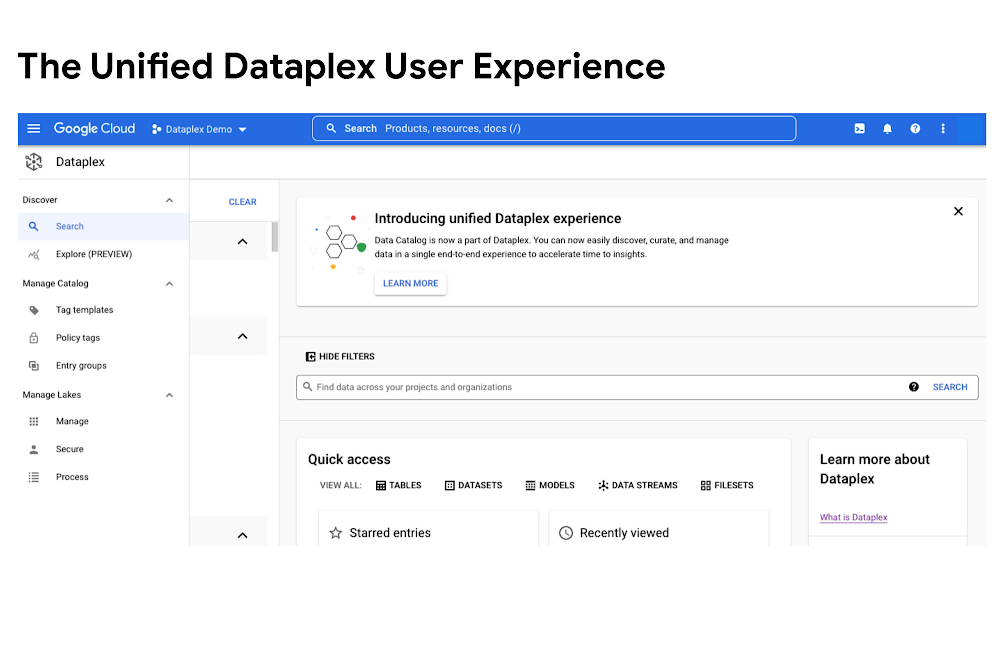
Google Cloud Data Heroes Series: Meet Tomi, a data engineer based in Germany and creator of the ‘Not So BigQuery Newsletter’

Google Cloud Data Heroes is a series where we share stories of the everyday heroes who use our data tools to do incredible things. Like any good superhero tale, we explore our Google Cloud Data Heroes’ origin stories, how they moved from data chaos to a data-driven environment, what projects and challenges they are overcoming now, and how they give back to the community. In this month’s edition, we’re pleased to introduce Tomi! Tomi grew up in Croatia, and is now residing in Berlin, Germany, where he currently works as a freelance Google Cloud data engineer. In this role, he regularly uses BigQuery. Tomi’s familiarity with BigQuery and his passion for Google Cloud led him to creating the weekly newsletter Not So BigQuery, where he discusses the latest data-related information from the GCP world.  Additionally, he also works for one of the largest automotive manufacturers in Germany as an analyst. When not in front of the keyboard, Tomi enjoys walking with his dog and his girlfriend, going to bakeries, or spending a night watching television.When were you introduced to the cloud, tech, or data field? What made you pursue this in your career? I always struggled with the question ‘what do you want to do in your life?. I attended school at Zagreb University of Applied Science for my information technology studies degree, but I was still unsure if I should become a developer, data engineer or something completely different.A couple of years into working as a junior IT Consultant, I stumbled upon a job advertisement looking for a Data Analyst/Scientist. Back then, finding out that you can get paid to just work with data all day sounded mind-blowing to me. A dream job.I immediately applied for the role and started learning about the skills needed. This is also where I gained my first experience with the Cloud as I signed up for a Google Cloud Platform free trial in February 2018. On the platform, there was a blog post describing how to run Jupyter notebooks in the Cloud. It interested me, and I went ahead and created my very first Compute Engine instance in Google Cloud Platform.I didn’t get the job I initially applied for, but this was the trigger for me that set things in motion and got me to where I am now.What courses, studies, degrees, or certifications were instrumental to your progression and success in the field? In your opinion, what data skills or competencies should data practitioners be focusing on acquiring to be successful in 2022 and why? Looking back at my university days, I really enjoyed the course about databases, which was partially because I had a really great teacher, but also because this was the first time I got to do something which catered to my then still-unknown data-nerdy side.In 2019, I got my Google Cloud Certified Associate Cloud Engineer Certification which was a challenging and rewarding entry-level certification for Google Cloud. I would recommend considering getting one of these as a way of focusing one’s learning.One major change I’ve observed since working in the data field is the ongoing transition from on-prem to cloud and serverless. I remember a story from my early consulting days working in an IT operations team, when there was a major incident caused by an on-prem server outage. At some point one frustrated colleague said something like, ‘why do we even have to have servers? Why can’t it just *run* somehow?’ What sounded like a bit of a silly question back then turned out to be quite ‘visionary’ with all the serverless and cloud-based tech we have today.What drew you to Google Cloud? Tell us about that process, what you’re most proud of in this area, and why you give back to the community? There is this great newsletter on Google Cloud Platform called GCP Weekly, run by a data community member named Zdenko Hrček that I really like. However, since the GCP ecosystem is growing at a rapid pace there are sometimes just too many news and blogs in a single week. I really struggled to catch up with all the new product updates and tutorials. That’s when I had the idea: ‘what if there would be a shorter newsletter with only news about BigQuery and other data-related tools’? Fast forward to today, my Not So BigQuery newsletter has more than 220 subscribers.I was also inspired by the awesome content created by Priyanka Vergadia, Staff Developer Advocate at Google Cloud, such as her Sketchnotes series. I created the GCP Data Wiki, which is a public Notion page with cards for every database/storage service in GCP with useful details such as links to official docs, Sketchnotes and more.What are 1-2 of your favorite projects you’ve done with Google Cloud’s data products? One of my first projects built with Google Cloud products was an automated data pipeline to get track data from the official Spotify API. I was looking for a data project to add to my portfolio and found out that Spotify lets you query their huge library via a REST API. This later evolved into a fully-serverless pipeline running on Google Cloud Functions and BigQuery. I also wrote a blog post about the whole thing, which got 310 claps on Medium.Additionally, the Not So BigQuery newsletter I created is actually powered by a tool I built using Google Sheets and Firebase (Functions). I have a Google Sheet where I pull in the news feed sections from sources such as the Google Cloud Blog and Medium. Using the built-in Sheets formulas such as IMPORTFEED and FILTER, I built a keyword-based article curation algorithm pre-selecting the articles to include in the next issue of the newsletter. Then my tool called crssnt (pronounced as the french pastry) takes the data from the Google Sheet and displays it in the newsletter. If you are curious how the Google Sheet looks like, you can check it out here.What are your favorite Google Cloud Platform data products within the data analytics, databases, and/or AI/ML categories? What use case(s) do you most focus on in your work? What stands out about GCP’s offerings?My favorite is BigQuery but I’m also a huge fan of Firestore. BigQuery is my tool of choice for pretty much all of my data warehouse needs (for both personal and client projects). What really stood out to me for me is the ease of use when it comes to setting up new databases from scratch and getting first results in the form of e.g. a Data Studio dashboard built on top of a BigQuery table. Similarly, I always go back to Firestore whenever I have an idea about some new front-end project since it’s super easy to get started and gives me a lot of flexibility.From similar non-Google products, I used Snowflake a while ago but didn’t find the user interface nearly as intuitive and user-friendly as BigQuery.What’s next for you in life? It’s going to be mostly ‘more of the same’ for me: as a data nerd, there is always something new to discover and learn. My overall message to readers would be to try to not worry too much about fitting into predefined career paths, job titles and so on, and just do your thing. There is always more than one way of doing things and reaching your goals. Want to join the Data Engineer Community?Register for the Data Engineer Spotlight on July 20th, where attendees have the chance to learn from four technical how-to sessions and hear from Google Cloud Experts on the latest product innovations that can help you manage your growing data. Begin your own Data Hero journeyReady to embark on your Google Cloud data adventure? Begin your own hero’s journey with GCP’s recommended learning path where you can achieve badges and certifications along the way. Join the Cloud Innovators program today to stay up to date on more data practitioner tips, tricks, and events.If you think you have a good Data Hero story worth sharing, please let us know! We’d love to feature you in our series as well.Related ArticleGoogle Cloud Data Heroes Series: Meet Francisco, the Ecuadorian American founder of Direcly, a Google Cloud PartnerIn the Data Heroes series we share stories of people who use data analytics tools to do incredible things. In this month’s edition, Meet …Read Article
Quelle: Google Cloud Platform

Using Google Kubernetes Engine’s GPU sharing to search for neutrinos

Editor’s note: Today we hear from the San Diego Supercomputer Center (SDSC) and University of Wisconsin-Madison about how GPU sharing in Google Kubernetes Engines is helping them detect neutrinos at the South Pole with the gigaton-scale IceCube Neutrino Observatory.IceCube Neutrino Observatory is a detector at the South Pole designed to search for nearly massless subatomic particles called neutrinos. These high-energy astronomical messengers provide information to probe events like exploding stars, gamma-ray bursts, and cataclysmic phenomena involving black holes and neutron stars. Scientific computer simulations are run on the sensory data that IceCube collects on neutrinos to pinpoint the direction of detected cosmic events and improve their resolution.The most computationally intensive part of the IceCube simulation workflow is the photon propagation code, a.k.a. ray-tracing, and that code can greatly benefit from running on GPUs. The application is high throughput in nature, with each photon simulation being independent of the others. Apart from the core data acquisition system at the South Pole, most of IceCube’s compute needs are served by an aggregation of compute resources from various research institutions all over the world, most of which use the Open Science Grid (OSG) infrastructure as their unifying glue. GPU resources are relatively scarce in the scientific resource provider community. In 2021, OSG had only 6M GPU hours vs 1800M CPU core hours in its infrastructure. The ability to expand the available resource pool with cloud resources is thus highly desirable.The SDSC team recently extended the OSG infrastructure to effectively use Kubernetes-managed resources to support IceCube compute workloads on the Pacific Research Platform (PRP). The service manages dynamic provisioning in a completely autonomous fashion by implementing horizontal pilot pod autoscaling based on the queue depth of the IceCube batch system. Unlike on-premises systems, Google Cloud offers the benefits of elasticity (on-demand scaling) and cost efficiency (only pay for what gets used). We needed a flexible platform that can avail these benefits to our community. We found Google Kubernetes Engine (GKE) to be a great match for our needs due to its support for auto-provisioning, auto-scaling, dynamic scheduling, orchestrated maintenance, job API and fault tolerance, as well as support for co-mingling of various machine types (e.g. CPU + GPU and on-demand + Spot) in the same cluster and up to 15,000 nodes per cluster.While IceCube’s ray-tracing simulation greatly benefits from computing on the GKE GPUs, it still relies on CPU compute for feeding the data to the GPU portion of the code. And GPUs have been getting faster at a much higher rate than CPUs have! With the advent of the NVIDIA V100 and A100 GPUs, the IceCube code is now CPU-bound in many configurations. By sharing a large GPU between multiple IceCube applications, the IceCube ray-tracing simulation again becomes GPU-bound, and therefore we get significantly more simulation results from the same hardware. GKE has native support for both simple GPU time-sharing and the more advanced A100 Multi-Instance GPU (MIG) partitioning, making it incredibly easy for IceCube — and OSG at large — to use.To leverage the elasticity of the Google Cloud, we fully relied on GKE horizontal node auto-scaling for provisioning and de-provisioning GKE compute resources. Whenever there were worker pods that could not be started, the auto-scaler provisioned more GKE nodes, up to a set maximum. Whenever a GKE node was unused, the auto-scaler de-provisioned it to save costs.Performance resultsUsing Google Cloud GPU resources was very simple through GKE. We used the same setup we were already using on the on-prem PRP Kubernetes cluster, simply pointing our setup to the new cluster.After the initial setup, IceCube was able to efficiently use Google Cloud resources, without any manual intervention by the supporting SDSC team beyond setting the auto-scaling limits. This was a very welcome change from other cloud activities the SDSC team has performed on behalf of IceCube and others, that required active management of provisioned resources.AutoscalingThe GKE auto-scaling for autonomous provisioning and de-provisioning of cloud resources worked as advertised, closely matching the demand from IceCube users, as seen in Fig. 1. We were particularly impressed by GKE’s performance in conjunction with GPU sharing; the test run shown used seven A100 MIG partitions per GPU.Fig. 1: Monitoring snapshot of the unconstrained GKE auto-scaling test run.GPU sharingBoth full-GPU and shared-GPU Kubernetes nodes with A100, V100 and T4 GPUs were provisioned, but IceCube jobs did not differentiate between them, since all provisioned resources met the jobs’ minimum requirements.We assumed that GPU sharing benefits would vary based on the CPU-to-GPU ratio of the chosen workflow, so during this exercise we picked one workflow from each extreme. IceCube users can choose to speed up the GPU-based ray-tracing compute of some problems by, roughly speaking, increasing the size of the target for the photons by some factor. For example, setting oversize=1 gives the most precise simulation, and oversize=4 gives the fastest. Faster compute (of course) results in a higher CPU-to-GPU ratio. The fastest oversize=4 workload benefitted the most from GPU sharing. As can be seen from Fig. 2, IceCube oversize=4 jobs cannot make good use of anything faster than a NVIDIA T4. Indeed, even for the low-end T4 GPU, sharing increases the job throughput by about 40%! For the A100 GPU, GPU sharing gets us a 4.5x throughput increase, which is truly transformational. Note that MIG and “plain” GPU sharing provide comparable throughput improvements, but MIG comes with much stronger isolation guarantees, which would be very valuable in a multi-user setup.Fig. 2: Number of IceCube oversize=4 jobs per hour, grouped by GPU setup.The more demanding oversize=1 workload makes much better use of the GPUs, so we observe no job throughput improvement for the older T4 and V100 GPUs. The A100 GPU, however, is still too powerful to be used as a whole, and GPU sharing gives us almost a 2x throughput improvement here, as illustrated in Fig. 3.Fig. 3: Number of IceCube oversize=1 jobs per day, grouped by GPU setup.GPU sharing of course increases the wallclock time needed by any single job to run to completion. This is however not a limiting factor for IceCube, since the main objective is to produce the output of thousands of independent jobs, and the expected timeline is measured in days, not minutes. Job throughput and cost effectiveness are therefore much more important than compute latency.Finally, we would like to stress that most of the used resources were provisioned on top of Spot VMs, making them significantly cheaper than their on-demand equivalents. GKE gracefully handled any preemption, making this mode of operation very cost effective.Lessons learnedGKE with GPU sharing has proven to be very simple to use, given that our workloads were already Kubernetes-ready. From a user point of view, there were virtually no differences from the on-prem Kubernetes cluster they were accustomed to.The benefits of GPU sharing obviously depend on the chosen workloads, but at least for IceCube it seems to be a necessary feature for the latest GPUs, i.e. the NVIDIA A100. Additionally, a significant fraction of IceCube jobs can benefit from GPU sharing even for lower-end T4 GPUs.When choosing the GPU-sharing methodology, we definitely prefer MIG partitioning. While less flexible than time-shared GPU sharing, MIG’s strong isolation properties make management of multi-workload setups much more predictable. That said, “plain” GPU sharing was still more than acceptable, and was especially welcome on GPUs that lack MIG support.In summary, the GKE shared-GPU experience was very positive. The observed benefits of GPU sharing in Kubernetes were an eye-opener and we plan to make use of it whenever possible.Want to learn more about sharing GPUs on GKE? Check out this user guide.Related ArticleTurbocharge workloads with new multi-instance NVIDIA GPUs on GKEYou can now partition a single NVIDIA A100 GPU into up to seven instances and allocate each instance to a single Google Kubernetes Engine…Read Article
Quelle: Google Cloud Platform

Performance considerations for loading data into BigQuery

It is not unusual for customers to load very large data sets into their enterprise data warehouse. Whether you are doing an initial data ingestion with hundreds of TB of data or incrementally loading from your systems of record, performance of bulk inserts is key to quicker insights from the data. The most common architecture for batch data loads uses Google Cloud Storage(Object storage) as the staging area for all bulk loads. All the different file formats are converted into an optimized Columnar format called ‘Capacitor’ inside BigQuery.This blog will focus on various file types and data loading tools for best performance. Data files that are uploaded to BigQuery, typically come in Comma Separated Values(CSV), Avro, Parquet, JSON, ORC formats. We are going to use a large dataset to compare and contrast each of these file formats. We will explore loading efficiencies of compressed vs. uncompressed data for each of these file formats. Data can be loaded into BigQuery using multiple tools in the GCP ecosystem. You can use the Google Cloud console, bq load command, using the BigQuery API or using the client libraries. We will also compare and contrast each loading mechanism for the same dataset. This blog attempts to elucidate the various options for bulk data loading into BigQuery and also provides data on the performance for each file-type and loading mechanism.Introduction There are various factors you need to consider when loading data into BigQuery. Data file formatData compressionTool used to load dataLevel of parallelization of data loadSchema autodetect ‘ON’ or ‘OFF’Data file formatBulk insert into BigQuery is the fastest way to insert data for speed and cost efficiency. Streaming inserts are however more efficient when you need to report on the data immediately. Today data files come in many different file types including comma separated(CSV), json, parquet, avro  to name a few. We are often asked how the file format matters and whether there are any advantages in choosing one file format over the other. CSV files (comma-separated values) contain tabular data with a header row naming the columns. When loading data one can parse the header for column names. When loading from csv files one can use the header row for schema autodetect to pick up the columns. With schema autodetect set to off, one can skip the header row and create a schema manually, using the column names in the header. CSV files can use other field separator/newline characters too as a separator, since many data outputs already have a comma in the data. You cannot store nested or repeated data in CSV file format.JSON (JavaScript object notation) data is stored as a key-value pair in a semi structured format. JSON is preferred as a file type because it can store data in a hierarchical format. The schemaless nature of json data rows gives the flexibility to evolve the schema and thus change the payload. JSON and XML formats are user-readable, but JSON documents are typically much smaller than XML. REST-based web services use json over other file types.Parquet is a column-oriented data file format designed for efficient storage and retrieval of data.  Parquet compression and encoding is very efficient and provides improved performance to handle complex data in bulk.Avro: The data is stored in a binary format and the schema is stored in JSON format. This helps in minimizing the file size and maximizes efficiency. Avro has reliable support for schema evolution by managing added, missing, and changed fields. From a data loading perspective we did various tests with millions to hundreds of billions of rows with narrow to wide column data .We have done this test with a public dataset named `bigquery-public-data:worldpop.population_grid_1km`. We used 4000 flex slots for the test and the number of loading slots is limited to the number of slots you have allocated for your environment, though the load slots do not use all of the slots you throw at it.. Schema Autodetection was set to ‘NO’. For the parallelization of the data files each file should typically be less than 256MB for faster throughput and here is a summary of our findings:Do I compress the data? Sometimes batch files are compressed for faster network transfers to the cloud. Especially for large data files that are being transferred, it is faster to compress the data before sending over the cloud Interconnect or VPN connection. In such cases is it better to uncompress the data before loading into BigQuery? Here are the tests we did for various file types with different compression algorithms.Shown results are the average of five runs:How do I load the data?There are various ways to load the data into BigQuery. You can use the Google Cloud Console, command line, Client Library(shown python here) or use the Direct API call. We compared these data loading techniques and compared the efficacy of each method. Here is a comparison of the timings for each method. You can also see that Schema Autodetect works very well, where there are no datatype quality issues in the source data and you are consistently getting the same columns from a data sourceConclusionThere is no advantage in loading time when the source file is in compressed format. In fact for the most part uncompressed data loads in the same or faster time than compressed data. We noticed that for csv and avro file types you do not need to uncompress for faster load times. For other file types including parquet and json it takes longer to load the data when the file is compressed. Decompression is a CPU bound activity and your mileage varies based on the amount of load slots assigned to your load job. Data loading slots are different from the data querying slots. For compressed files, you should parallelize the load operation, so as to make sure that data loads are efficient. Split the data files to 256MB or less to avoid spilling over the uncompression task to disk.From a performance perspective avro, csv and parquet files have similar load times. Use the command line to load larger volumes of data for the most efficient data loading. Fixing your schema does load the data faster than schema autodetect set to ‘ON’. Regarding ETL jobs, it is faster and simpler to do your transformation inside BigQuery using SQL, but if you have complex transformation needs that cannot be done with SQL, use Dataflow for unified batch and streaming, Dataproc for open source based pipelines, or Cloud Data Fusion for no-code / low-code transformation needs.To learn more about how Google BigQuery can help your enterprise, try out Quickstarts page here.Disclaimer: These tests were done with limited resources for BigQuery in a test environment during different times of the day with noisy neighbors, so the actual timings and the number of rows might not be reflective of your test results. The numbers provided here are for comparison sake only, so that you can choose the right file types, compression and loading technique for your workload. Related ArticleLearn how BI Engine enhances BigQuery query performanceThis blog explains how BI Engine enhances BigQuery query performance, different modes in BI engine and its monitoring.Read Article
Quelle: Google Cloud Platform

Introducing model co-hosting to enable resource sharing among multiple model deployments on Vertex AI

When deploying models to the Vertex AI prediction service, each model is by default deployed to its own VM. To make hosting more cost effective, we’re excited to introduce model co-hosting in public preview, which allows you to host multiple models on the same VM, resulting in better utilization of memory and computational resources. The number of models you choose to deploy to the same VM will depend on model sizes and traffic patterns, but this feature is particularly useful for scenarios where you have many deployed models with sparse traffic.Understanding the Deployment Resource PoolCo-hosting model support introduces the concept of a Deployment Resource Pool, which groups together models to share resources within a VM. Models can share a VM if they share an endpoint, but also if they are deployed to different endpoints. For example, let’s say you have four models and two endpoints, as shown in the image below.Model_A, Model_B, and Model_C are all deployed to Endpoint_1 with traffic split between them. And Model_D is deployed to Endpoint_2, receiving 100% of the traffic for that endpoint. Instead of having each model assigned to a separate VM, we can group Model_A and Model_B to share a VM, making them part of DeploymentResourcePool_X. We can also group models that are not on the same endpoint, so Model_C and Model_D can be hosted together in DeploymentResourcePool_Y. Note that for this first release, models in the same resource pool must also have the same container image and version of the Vertex AI pre-built TensorFlow prediction containers. Other model frameworks and custom containers are not yet supported.Co-hosting models with Vertex AI PredictionsYou can set up model co-hosting in a few steps. The main difference is that you’ll first create a DeploymentResourcePool, and then deploy your model within that pool. Step 1: Create a DeploymentResourcePoolYou can create a DeploymentResourcePool with the following command. There’s no cost associated with this resource until the first model is deployed.code_block[StructValue([(u’code’, u’PROJECT_ID={YOUR_PROJECT}rnREGION=”us-central1″rnVERTEX_API_URL=REGION + “-aiplatform.googleapis.com”rnVERTEX_PREDICTION_API_URL=REGION + “-prediction-aiplatform.googleapis.com”rnMULTI_MODEL_API_VERSION=”v1beta1″rn rn# Give the pool a namernDEPLOYMENT_RESOURCE_POOL_ID=”my-resource-pool”rn rnCREATE_RP_PAYLOAD = {rn “deployment_resource_pool”:{rn “dedicated_resources”:{rn “machine_spec”:{rn “machine_type”:”n1-standard-4″rn },rn “min_replica_count”:1,rn “max_replica_count”:2rn }rn },rn “deployment_resource_pool_id”:DEPLOYMENT_RESOURCE_POOL_IDrn}rnCREATE_RP_REQUEST=json.dumps(CREATE_RP_PAYLOAD)rn rn!curl \rn-X POST \rn-H “Authorization: Bearer $(gcloud auth print-access-token)” \rn-H “Content-Type: application/json” \rnhttps://{VERTEX_API_URL}/{MULTI_MODEL_API_VERSION}/projects/{PROJECT_ID}/locations/{REGION}/deploymentResourcePools \rn-d ‘{CREATE_RP_REQUEST}”), (u’language’, u”), (u’caption’, <wagtail.wagtailcore.rich_text.RichText object at 0x3e467adcff10>)])]Step 2: Create a modelModels can be imported to the Vertex AI Model Registry at the end of a custom training job, or you can upload them separately if the model artifacts are saved to a Cloud Storage bucket. You can upload a model through the UI or with the SDK using the following command:code_block[StructValue([(u’code’, u”# REPLACE artifact_uri with GCS path to your artifactsrnmy_model = aiplatform.Model.upload(display_name=’text-model-1′,rn artifact_uri=u2019gs://{YOUR_GCS_BUCKET}u2019,rn serving_container_image_uri=’us-docker.pkg.dev/vertex-ai/prediction/tf2-cpu.2-7:latest’)”), (u’language’, u”), (u’caption’, <wagtail.wagtailcore.rich_text.RichText object at 0x3e464c9e0f90>)])]When the model is uploaded, you’ll see it in the model registry. Note that the deployment status is empty since the model hasn’t been deployed yet.Step 3: Create an endpointNext, create an endpoint via the SDK or the UI. Note that this is different from deploying a model to an endpoint.endpoint = aiplatform.Endpoint.create(‘cohost-endpoint’)When your endpoint is created, you’ll be able to see it in the console.Step 4: Deploy Model in a Deployment Resource PoolThe last step before getting predictions is to deploy the model within the DeploymentResourcePool you created.code_block[StructValue([(u’code’, u’MODEL_ID={MODEL_ID}rnENDPOINT_ID={ENDPOINT_ID}rn rnMODEL_NAME = “projects/{project_id}/locations/{region}/models/{model_id}”.format(project_id=PROJECT_ID, region=REGION, model_id=MODEL_ID)rnSHARED_RESOURCE = “projects/{project_id}/locations/{region}/deploymentResourcePools/{deployment_resource_pool_id}”.format(project_id=PROJECT_ID, region=REGION, deployment_resource_pool_id=DEPLOYMENT_RESOURCE_POOL_ID)rn rnDEPLOY_MODEL_PAYLOAD = {rn “deployedModel”: {rn “model”: MODEL_NAME,rn “shared_resources”: SHARED_RESOURCErn },rn “trafficSplit”: {rn “0”: 100rn }rn}rnDEPLOY_MODEL_REQUEST=json.dumps(DEPLOY_MODEL_PAYLOAD)rnpp.pprint(“DEPLOY_MODEL_REQUEST: ” + DEPLOY_MODEL_REQUEST)rn rn!curl -X POST \rn-H “Authorization: Bearer $(gcloud auth print-access-token)” \rn-H “Content-Type: application/json” \rnhttps://{VERTEX_API_URL}/{MULTI_MODEL_API_VERSION}/projects/{PROJECT_ID}/locations/{REGION}/endpoints/{ENDPOINT_ID}:deployModel \rn-d ‘{DEPLOY_MODEL_REQUEST}”), (u’language’, u”), (u’caption’, <wagtail.wagtailcore.rich_text.RichText object at 0x3e464c9e0c90>)])]When the model is deployed, you’ll see it ready in the console. You can deploy additional models to this same DeploymentResourcePool for co-hosting using the same endpoint we created already, or using a new endpoint.Step 5: Get a predictionOnce the model is deployed, you can call your endpoint in the same way you’re used to.x_test= [‘The movie was spectacular. Best acting I’ve seen in a long time and a great cast. I would definitely recommend this movie to my friends!’]endpoint.predict(instances=x_test)What’s nextYou now know the basics of how to co-host models on the same VM. For an end to end example, check out this codelab, or refer to the docs for more details. Now it’s time for you to start deploying some models of your own!Related ArticleSpeed up model inference with Vertex AI Predictions’ optimized TensorFlow runtimeThe Vertex AI optimized TensorFlow runtime can be incorporated into serving workflows for lower latency predictions.Read Article
Quelle: Google Cloud Platform

Cloud SQL – SQL Server Performance Analysis and Query Tuning

The following blog covers popular performance analysis tools and technologies database administrators can use to tune and optimize Cloud SQL for SQL Server. Common performance challenges are described in each section along with tools and strategies to analyze, address and remediate them. After reviewing this blog, consider applying the tools and processes detailed in each section to a non-production database in order to gain a deeper understanding of how they can help you to manage and optimize your databases. We will also publish a follow up blog that will walk you through common performance issues and how to troubleshoot and remediate those using the tools and processes described here.1. Getting Started: Connecting to your Cloud SQL for SQL Server instance.The most common use cases for connecting to Cloud SQL include connecting from a laptop over VPN and using a jump host in GCP. SQL Server DBAs who connect from a local laptop over VPN using SQL Server Management Studio (SSMS) should review this Quickstart document for connecting to a Cloud SQL instance that is configured with a private IP address. DBAs may also prefer to connect to a single jump host for centralized management of multiple Cloud SQL for SQL Server instances. In this scenario, a Google Compute Engine (GCE) VM is provisioned and DBAs use a Remote Desktop Protocol (RDP) tool to connect to the jump host and manage their Cloud SQL databases. For a comprehensive list of options on connecting to Cloud SQL, see connecting to Cloud SQL for SQL Server. 2. Activity Monitoring: What’s running right now? When responding to urgent support calls, DBAs have an immediate need to determine what is currently running on the instance.  Historically, DBAs have relied on system stored procedures such as sp_Who and sp_Who2 to support triage and analysis. To determine what’s running right now, consider installing Adam Machanic’s sp_WhoIsActive stored procedure. To view currently running statements and to obtain details on the plans, use the statement below. Note that in the following example, the procedure sp_WhoIsActive has been installed on the dbo schema of the dbtools database. EXEC dbtools.dbo.sp_WhoIsActive @get_plans=1Also, see Brent Ozar’s sp_BlitzFirst stored procedure, which is included in the SQL-Server-First-Responder-Kit. Review the documentation for examples. 3. Optimizing queries using the SQL Server Query Store.Query optimization is best to be performed proactively  as a weekly DBA checklist item.  The SQL Server Query Store feature can help with this and provides DBAs with query plans, history and useful performance metrics. Before starting the SQL Server Query Store, it is a good idea to review the following Microsoft SQL Server Performance Monitoring article: Monitoring performance by using the Query Store . Query Store is enabled on a database level and must be enabled for each user database. See the example below for how to enable Query Store. ALTER DATABASE <<DBNAME>>SET QUERY_STORE = ON (WAIT_STATS_CAPTURE_MODE = ON);After enabling Query Store, review the Query Store configuration using SSMS. Right-click on the database and view Query Store properties. Review the Microsoft article Monitoring performance by using the Query Store for more information on properties and settings. Screenshot: Query Store has been enabled on the AdventureWorksDW2019 database.After enabling Query Store on a busy instance, query data will normally be available for review within a few minutes. Alternatively, run a few test queries to generate data for analysis. Next, expand the Query Store node to explore available reports.In the example below, I selected “Top Resource Consuming Queries”. I then sorted the table by total duration and reviewed the execution plan for the top resource consuming query. In reviewing the execution plan I noted that a table scan was occurring. I was then able to remediate the issue by asking the user to modify their query to select specific columns rather than selecting all the columns, and then added a non-clustered index to the underlying table to include the required columns.Example Index Change:code_block[StructValue([(u’code’, u’CREATE NONCLUSTERED INDEX NCIX_dbo_scenario1_LastName_INCLUDE_FirstName_BirthDatern ON [dbo].[scenario1] (LastName) INCLUDE (FirstName, BirthDate); rnGO’), (u’language’, u”), (u’caption’, <wagtail.wagtailcore.rich_text.RichText object at 0x3ec8a528d690>)])]To track a query over time, right-click the query and select “Track Query”.Note that the plans for before and after the index change are shown below.Select both plans, then choose “Compare Plans” to view pre and post plan changes.SQL Server Query Store is a helpful built-in performance tuning tool that is available for Cloud SQL DBAs to capture, analyze and tune T-SQL statements. It makes sense to spend time learning about how Query Store can help you manage and optimize your SQL Server databases.4. Analyzing instance and database health, configuration and performance.The SQL Server Community offers many free tools and scripts for reviewing and analyzing SQL Server instances and databases. A few popular script resources are noted below. Glen Berry’s SQL Server Diagnostic Queries are useful for assessing on-prem instances when planning for a migration, and analyzing configurations and performance once databases are running in GCP.  For more information on how to use the SQL Server Diagnostic Queries, and for help interpreting the results, review Glen’s YouTube videos.Brent Ozar’s SQL-Server-First-Responder-Kit is another popular community tool used to quickly assess and analyze SQL Server instances. Note that Cloud SQL for SQL Server does not support installing objects in the master database, and it is recommended that a separate database is created for the scripts. Many DBAs create a tools database (for example: dbtools), and install scripts and procedures in that database. Review the documentation and Brent’s how-to videosfor tips on installing and using the kit. 5. Configuration and performance levers to reduce locking and blocking.Performance problems related to locking and blocking may be reduced by scaling up the instance and optimizing database objects like tables, queries and stored procedures. While increasing instance performance may provide quick wins in the short-term, optimizing SQL and application code results in better stability and performance over the long term.Instance Cores and Storage CapacityIncreasing cores and storage capacity, also known as scaling up, has an immediate effect on IO throughput and performance, and many workload performance issues may be mitigated by increasing CPU and Storage configuration settings. Disk performance is based on the disk size and the number of vCPUs. Add more storage space and vCPUs to increase IOPS and throughput.Read Committed Snapshot Isolation (RCSI) If you find yourself adding NO LOCK to your queries in an attempt to reduce contention and speed things up, it’s probably a good idea to take a look at Read Committed Snapshot Isolation. When READ_COMMITTED_SNAPSHOT is turned on, SQL Server Engine uses row versioning instead of locking.  For more information, see Kendra Little’s blog post on How to Choose Between RCSI and Snapshot Isolation Levels to determine if RCSI is right for your database workloads.Forced ParameterizationIf you run across an application that generates a lot of dynamic SQL or executes SQL without parameters, you may see a lot of CPU time wasted on creating new plans for SQL queries. In some cases, Forced Parameterization can help your database performance when you are not able to change or influence application coding standards. For more on forced parameterization and how it can be applied, review the following link:  SQL Server Database Parameterization option and its Query Performance effects  6. Managing Indexes and Statistics: SQL Server maintenanceOla Hallengren’s SQL Server Maintenance Solution is a SQL Server Community standard database maintenance solution. In an on-premises or GCE environment, a DBA may choose to install the entire maintenance solution, including backup scripts. Since backups are handled internally by Cloud SQL, a DBA may choose to install only the Statistics and Indexing procedures and supporting objects. Visit https://ola.hallengren.com/ to learn more about the solution, and take time to review the associated scripts, instructions, documentation and examples of how to install and use the SQL Server Maintenance Solution.ConclusionProactively managing and tuning your Cloud SQL SQL Server databases enables DBAs to spend less time on production support calls and increases the performance, efficiency and scalability of databases. Many of the tools and recommendations noted in this blog are also applicable to SQL Server databases running on GCE. Once you become familiar with the tools and processes featured in this blog, consider integrating them into your database workflows and management plans.Related ArticleCloud SQL for SQL Server: Database administration best practicesCloud SQL for SQL Server is a fully-managed relational database service that makes it easy to set up, maintain, manage, and administer SQ…Read Article
Quelle: Google Cloud Platform