Kategorie: Google Cloud Platform

Get to know the top 3 teams of the Google Cloud Hackathon Singapore

Google Cloud hackathonOn 10th April 2022, Google Cloud launched the first Singapore Google Cloud Hackathon, where startup teams were tasked to build solutions for either the topics of Sustainability, Artificial Intelligence, Automation or the New Normal, to create innovative solutions and have the opportunity to win prizes. From April to 10th June, Google Cloud worked with hackathon entrants through the solutioning process from ideation to prototyping to the final pitch. The hackathon saw incredible response with 40 startup teams competing for a top 5 spot. The top 5 teams were invited to pitch live at the Google Asia Pacific Singapore Campus and presented to a panel of judges that consisted of experts in the startup ecosystem and technology leaders across APAC in Google. The top 3 teams also continued to receive mentorship opportunities with Google Cloud and startup experts.  Top 3 teamsRead on to learn more about the top 3 startup teams:Team Empathly – 2nd Runner UpCofounders Timothy Liau, Jamie Yau and Rachel Tan personally experienced hate speech and witnessed discrimination in online communities. The available content filters and manual moderation solutions, which they found to be very expensive, only focused on damage control after the hateful comment has been sent. Out of a desire to prevent the toxic behavior at its source, Empathly was born.Any platform with user-generated content — social media, games, marketplaces, dating apps and more — is susceptible to hate speech. Described as “The Grammarly for content moderation”, Empathly applies its AI that identifies distinct types of hate speech with context – to promote safer and more inclusive speech in workplaces and online platforms. Empathy is built on Cloud Run and Cloud Firestore.Empathly’s behavioral science advisory team includes Yale-NUS professor and expert in behavioral insights Dr. Jean Liu whose research focuses on how technological solutions require an appreciation of human behavior and the social context. They will focus their next few months on working closely with their early customers and building toward product-market-fit.Team Ambient Systems – 1st Runner UpIvan Damnjanović founded Ambient to help companies meet their decarbonization targets through data science innovation. The team consists of Ivan and Frey Liu, a fellow computer science masters student from National University of Singapore (NUS). Through Ambient’s platform, companies can access real time Big Data analytics for actionable decarbonisation through energy efficiency and trade-off optimization.In 2020, Ambient Systems was founded when Ivan proposed a software-based solution for managing complex indoor air quality challenges, such as airborne transmission of COVID and vertical farming climate conditions. Ivan’s patent in the AgriTech field helped Ambient secure a $100k investment from NUS to further pursue commercialization of the technology and help Singapore achieve its 30 by 30 agenda – to build Singapore’s “agri-food industry’s capability and capacity to produce 30% of our nutritional needs locally and sustainably by 2030”.Through the use of Google’s Firebase platform, the team was able to quickly build a fully functional prototype that garnered interest from investors and customers.Team Pomona – ChampionsAs harsh weather conditions continue to plummet agricultural yield, there is an increasing need for countries to improve food security through efficient agriculture and sustainable living. However, high operational costs and cyclical risks inhibit the growth of vertical farming in the agricultural industry.Team Pomona consists of Pang Jun Rong, Yuen Kah May, Teo Keng Swee, Nicole Lim Jia Yi, Tan Jie En, who are student entrepreneurs from Singapore Management University (SMU) Computer Science. They took motivation from their school’s efforts in sustainability and technology to form Pomona — a solution set on making food security more personal through the ownership of vegetables in commercial agricultural lifecycles.Pomona features a gamified de-fi agricultural platform to promote collective ownership of vertical farming agriculture, which enables profit-sharing between producers and consumers to hedge against operational risks. This was done through a hybrid decentralized microservice cloud architecture with Google Cloud, using blockchain technologies for “dVeg” digital tokens and conventional full-stack components for gamification with IoT integration, providing real-time interactive growth tracking for lifecycle traceability.Final wordsCongratulations to all of the teams and especially Empathy, Ambient Systems, and Pomona. We look forward to more events with startups in the future!
Quelle: Google Cloud Platform

Scaling heterogeneous graph sampling for GNNs with Google Cloud Dataflow

This blog presents an open-source solution to heterogeneous graph sub-sampling at scale using Google Cloud Dataflow (Dataflow). Dataflow is Google’s publicly available, fully managed environment for running large scale Apache Beam compute pipelines. Dataflow provides monitoring and observability out of the box and is routinely used to scale production systems to easily handle extreme datasets.This article will present the problem of graph sub-sampling as a pre-processing step for training a Graph Neural Network (GNN) using Tensorflow-GNN (TF-GNN), Google’s open-source GNN library.The following sections will motivate the problem, present an overview of the necessary tools including Docker, Apache Beam, Google Cloud Dataflow, TF-GNN Unigraph format, TF-GNN graph-sampler concluding with end-to-end tutorial using large heterogeneous citation network (OGBN-MAG) popular for GNN (node-prediction) benchmarking. We do not cover modeling or training with TF-GNN which is covered by the libraries’ documentation and paper.MotivationRelational datasets (datasets with graph structure) including data derived from social graphs, citation networks, online communities and molecular data continue to proliferate and applying Deep Learning methods to better model and derive insights from structured data are becoming more common. Even if a dataset is originally unstructured, it’s not uncommon to observe performance gains for ML tasks by inferring structure before applying deep learning methods through tools such as Grale (semi-supervised graph learning).Visualized below is a synthetic example visualizing a citation network in the same style as the popular OGBN-MAG dataset. The figure shows a heterogeneous graph – a relational dataset with multiple types of nodes (entities) and relationships (edges) between them. In the figure there are two entities, “Paper” and “Author”.  Certain authors “Write” specific papers defining a relation between “Author” entities and “Paper” entities. “Papers” commonly “cite” other “Papers” building a relationship between the “Paper” entities.For real world applications, the number of entities and relationships may be very large and complex and in most cases, it is impossible to load a complete dataset into memory on a single machine.A visualization of OGBN-MAG citation network as a heterogeneous graph. For a given relational dataset or heterogeneous graph, there are (potentially) multiple types of entities and various types of relationships between entities.Graph Neural Networks (GNNs or GCNs) are a fast growing suite of techniques for extending Deep Learning and Message Passing frameworks to structured data and Tensorflow GNN (TF-GNN) is Google’s Graph Neural Networks library built on the Tensorflow platform. TF-GNN defines native tensorflow objects, including tfgnn.GraphTensor, capable of representing arbitrary heterogeneous graphs, models and processing pipelines that can scale from academic to real world applications including graphs with millions of nodes and trillions of edges.Scaling GNN models to large graphs is difficult and an active area of research as real world structured data sets typically do not fit in the memory available on a single computer making training/inference using a GNN impossible on a single machine. A potential solution is to partition a large graph into multiple pieces, each of which can fit on a single machine and be used in concert for training and inference. As GNNs are based on message-passing algorithms, how the original graph is partitioned is crucial to model performance.While conventional Convolutional Neural Networks (CNNs) have regularity that can be exploited to define a natural partitioning scheme, kernels used to train GNNs potentially overlap the surface of the entire graph, are irregularly shaped and are typically sparse. While other approaches to scaling GCNs exist, including interpolation and precomputing aggregations, we focus on subgraph sampling: partitioning the graph into smaller subgraphs using random explorations to capture the structure of the original graph.In the context of this document, the graph sampler is a batch Apache Beam program that takes a (potentially) large, heterogeneous graph and a user-supplied sampling specification as input, performs subsampling, and writes tfgnn.GraphTensors to a storage system encoded for downstream TF-GNN training.Introduction to Docker, Beam, and Google Cloud DataflowApache Beam (Beam) is an open-source SDK for expressing compute intensive processing pipelines with support for multiple backend implementations. Google Cloud Platform (GCP) is Google’s cloud computing service, of which Dataflow is GCPs implementation for running Beam pipelines at scale. The two main abstractions defined by the Beam SDK arePipelines – computational steps expressed as a DAG (Directed Acyclic Graph)Runners – Environments for running pipelines using different types of controller/server configurations and optionsComputations are expressed as Pipelines using the Apache Beam SDK and the Runners define a compute environment. Specifically, Google provides a Beam Runner implementation called the DataflowRunner that connects to a GCP project (with user supplied credentials) and executes the Beam pipeline in the GCP environment. Executing a Beam pipeline in a distributed environment involves the use of “worker” machines, compute units that execute steps in the DAG. Custom operations defined using the Beam SDK must be installed and available on the worker machines and data communicated between workers must be able to be serialized/deserialized for inter-worker communication. In addition to the DataflowRunner, there exists a DirectRunner which enables users to execute Beam pipelines on local hardware and is typically used for development, verification, and testing.When clients use the DirectRunner to launch Beam pipelines, the compute environment of the pipeline mirrors the local host; libraries and data available on the users’ machine are available to the Beam work units. This is not the case when running in a distributed environment. Worker machines compute environments are potentially different from the host that dispatches the remote Beam pipeline. While this might be sufficient for Pipelines that only rely on python standard libraries, this is typically not acceptable for scientific computing which may rely on mathematical packages or custom definitions and bindings. For example, TFGNN defines Protocol Buffers (tensorflow/gnn/proto) whose definitions must be installed both on the client that initiates the Beam pipeline and the workers that execute the steps of the sampling DAG. One solution is to generate a Docker image that defines a complete TFGNN runtime environment that can be installed on Dataflow workers before Beam pipeline execution.Docker containers are widely used and supported in the open source community for defining portable virtualized run-time environments that can be isolated from other applications on a common machine. A Docker Container is defined as a running instance of a Docker Image (conceptually a read-only binary blob or template). Images are defined by a Dockerfile that enumerates the specifics of a desired compute environment. Users of a Dockerfile “build” a Docker Image which can be used and shared by other people who have Docker installed to instantiate the isolated compute environment. Docker images can be built locally with tools like the Docker CLI or remotely via Google Cloud Build (GCB). Docker images can be shared in public or private repositories such as Google Container Registry or Google Artifact Registry.TF-GNN provides a Dockerfile specifying an operating system along with a series of packages, versions and installation steps to set up a common, hermetic compute environment that any user of TF-GNN (with docker installed) can use. With GCP, TF-GNN users can build a TF-GNN docker image and push that image to an image repository that Dataflow workers can install prior to being scheduled by a Dataflow pipeline execution.Unigraph Data FormatThe TF-GNN graph sampler accepts graphs in a format called unigraph. Unigraph supports very large, homogeneous and heterogeneous graphs with variable numbers of node sets and edge sets (types). Currently, in order to use the graph sampler, users need to convert their graph to unigraph format.The unigraph format is backed by a text-formatted GraphSchema protocol buffer (proto) message file describing the full (unsampled) graph topology. The GraphSchema defines three main artifacts:context: Global graph featuresnode sets: Sets of nodes with different types and (optionally) associated featuresedge sets: the directed edges relating nodes in node setsFor each context, node set and edge set there is an associated “table” of ids and features which may be in one of many supported formats; CSV files, shared tf.train.Example protos in TFRecords containers and more. The location of each “table” artifact may be absolute or local to the schema. Typically, a schema and all “tables” live under the same directory which is dedicated to the graph’s data. Unigraph is purposefully simple to enable users to easily translate their custom data source into a unigraph format which the graph sampler and subsequently TF-GNN can consume.Once the unigraph is defined, the graph sampler requires two more configuration artifacts:The location of the unigraph GraphSchema messageA SamplingSpec protocol buffer message(Optional) Seed node-ids If provided, random explorations will begin from the specified “seed” node-ids only.The graph sampler generates subgraphs by randomly exploring the graph structure starting from a set of “seed nodes”. The seed nodes are either explicitly specified by the user or, if omitted, every node in the graph is used as a seed node which will result in one subgraph for every node in the graph. Exploration is done at scale, without loading the entire graph on a single machine through the use of the Apache Beam programming model and Dataflow engine.A SamplingSpec message is a graph sampler configuration that allows the user control how the sampler will explore the graph through edge sets and perform sampling on node sets (starting from seed nodes). The SamplingSpec is yet another text formatted protocol buffer message that enumerates sampling operations starting from a single `seed_op` operation.  Example: OGBN-MAG Unigraph FormatAs a clarifying example, consider the OGBN-MAG dataset, a popular, large, heterogeneous citation network containing the following node and edge sets:OGBN-MAG Node Sets”paper” contains 736,389 published academic papers, each with a 128-dimensional word2vec feature vector computed by averaging the embeddings of the words in its title and abstract.”field_of_study” contains 59,965 fields of study, with no associated features.”author” contains the 1,134,649 distinct authors of the papers, with no associated features”institution” contains 8740 institutions listed as affiliations of authors, with no associated features.OGBN-MAG Edge Sets”cites” contains 5,416,217 edges from papers to the papers they cite.”has_topic” contains 7,505,078 edges from papers to their zero or more fields of study.”writes” contains 7,145,660 edges from authors to the papers that list them as authors.”affiliated_with” contains 1,043,998 edges from authors to the zero or more institutions that have been listed as their affiliation(s) on any paper.This dataset can be described in unigraph with the following skeleton GraphSchema message:code_block[StructValue([(u’code’, u’node_sets {rn key: “author”rn u2026rn}rn..rnnode_sets {rn key: “paper”rn u2026rn}rnedge_sets {rn key: “affiliated_with”rn value {rn source: “author”rn target: “institution”rn u2026rn}rnu2026rnedge_sets {rn key: “writes”rn value {rn source: “author”rn target: “paper”rn u2026rn }rn}rnedge_sets {rn key: “written”rn value {rn source: “paper”rn target: “author”rn metadata {rn u2026rn extra {rn key: “edge_type”rn value: “reversed”rn }rn }rn }rn}’), (u’language’, u”), (u’caption’, <wagtail.wagtailcore.rich_text.RichText object at 0x3efa1bb95a10>)])]This schema omits some details (a full example is included in the TFGNN repository) but the outline is sufficient to show that the GraphSchema message merely enumerates the node types as collections of node_sets and the relationships between the node sets are defined by the edge_sets messages. Note the additional “written” edge set. This relation is not defined in the original dataset or manifested on persistent media. However, the “written” table specification defines a reverse relation creating a directed edge from papers back to authors as the transpose of the “writes” edge set. The tfgnn-sampler will parse the metadata.extra tuple and if the edge_type/reverse key-value pair is present, generate an additional PCollection of edges (relations) that swaps the sources and targets relative the relations expressed on persistent media.Sampling SpecificationA TF-GNN modeler would craft a SamplingSpec configuration for a particular task and model. For OGBN-MAG, one particular task is to predict the venue (journal or conference) that a paper from a test set is published at. The following would be a valid sampling specification for that task:code_block[StructValue([(u’code’, u’seed_op {rn op_name: “seed”rn node_set_name: “paper”rn}rnsampling_ops {rn op_name: “seed->paper”rn input_op_names: “seed”rn edge_set_name: “cites”rn sample_size: 32rn strategy: RANDOM_UNIFORMrn}rnsampling_ops {rn op_name: “paper->author”rn input_op_names: [“seed”, “seed->paper”]rn edge_set_name: “written”rn sample_size: 8rn strategy: RANDOM_UNIFORMrn}rnsampling_ops {rn op_name: “author->paper”rn input_op_names: “paper->author”rn edge_set_name: “writes”rn sample_size: 16rn strategy: RANDOM_UNIFORMrn}rnsampling_ops {rn op_name: “author->institution”rn input_op_names: “paper->author”rn edge_set_name: “affiliated_with”rn sample_size: 16rn strategy: RANDOM_UNIFORMrn}rnsampling_ops {rn op_name: “paper->field_of_study”rn input_op_names: [“seed”, “seed->paper”, “author->paper”]rn edge_set_name: “has_topic”rn sample_size: 16rn strategy: RANDOM_UNIFORMrn}’), (u’language’, u”), (u’caption’, <wagtail.wagtailcore.rich_text.RichText object at 0x3efa1bb95410>)])]This particular SamplingSpec may be visualized in plate notation showing the relationship between the node sets and relations in the sampling specification as:Visualization of a valid OGBN-MAG SamplingSpec for the node prediction challenge.In human-readable terms, this sampling specification may be described as the following sequence of steps:Use all entries in the “papers” node set as “seed” nodes (roots of the sampled subgraphs).Sample 16 more papers randomly starting from the “seed” nodes through the citation edge set. Call this sampled set “seed->paper”.For both the “seed” and “seed->paper” sets, sample 8 authors using the “written” edge set. Name the resulting set of sampled authors “paper->author”.For each author in the “paper->author” set, sample 16 institutions via the “affiliated_with” edge set.For each paper in the “seed”, “seed->paper” and “author->paper” sample 16 fields of study via the “has_topic” relation.Node vs. Edge AggregationCurrently, the graph sampler program takes an optional input flag edge_aggregation_method which can be set to either node or edge (defaults to edge). The edge aggregation method defines the edges that the graph sampler collects on a per-subgraph basis after random exploration.Using the edge aggregation method, the final subgraph will only include the edges traversed during random exploration. Using the node aggregation method, the final subgraph will contain all edges that have a source and target node in the set of nodes visited during exploration. As a clarifying example, consider a graph with three nodes {A, B, C} with directed edges as shown below.Example graph.Instead of random exploration, assume we perform a one-hop breadth first search exploration starting at seed-node “A”, traversing edges A → B and A → C. Using the edge aggregation method, the final subgraph would only retain edges A → B and A → C while the node aggregation would include A → B, A → C and the B → C edge. The example sampling paths along with the edge and node aggregation results are visualized below.Left: Example sampling path. Middle: Edge aggregation sampling result. Right: Node aggregation sampling result.The edge aggregation method is less expensive (time and space) than node aggregation yet node aggregation typically generates subgraphs with higher edge density. It has been observed in practice that node-based aggregation can generate better models during training and inference for some datasets.TF-GNN Graph Sampling with Google Cloud Dataflow OBGN-MAG: End-To-End ExampleThe graph sampler, Apache Beam program implementing heterogeneous graph sampling can be found in the TF-GNN open-source repository.While alternative workflows are possible, this tutorial assumes the user will be building Docker images and initiating a Dataflow job from a local machine with internet access.First install docker on a local host machine then checkout the tensorflow_gnn repository.code_block[StructValue([(u’code’, u’git clone https://github.com/tensorflow/gnn.git’), (u’language’, u”), (u’caption’, <wagtail.wagtailcore.rich_text.RichText object at 0x3efa1a40ac10>)])]The user will need the name of their GCP project (which we refer to as  GCP_PROJECT) and some sort of GCP credentials. Default application credentials are typical for developing and testing within an isolated project but for production systems, consider maintaining custom service account credentials. Default application credentials may be obtained by:code_block[StructValue([(u’code’, u’gcloud auth application-default login’), (u’language’, u”), (u’caption’, <wagtail.wagtailcore.rich_text.RichText object at 0x3efa1a40a990>)])]On most systems, this command will download the access credentials to the following location: ~/.config/gcloud/application_default.json.Assuming the location of the cloned TF-GNN repository is ~/gnn, The TF-GNN docker image can be built and pushed the a GCP container registry with the following:code_block[StructValue([(u’code’, u’docker build ~/gnn -t tfgnn:latest gcr.io/${GCP_PROJECT}/tfgnn:latestrndocker push gcr.io/${GCP_PROJECT}/tfgnn:latest’), (u’language’, u”), (u’caption’, <wagtail.wagtailcore.rich_text.RichText object at 0x3efa2d1a46d0>)])]Building and pushing the image may take some time. To avoid the local build/push, the image can be built directly from a local Dockerfile remotely using Google Cloud Build.Get the OGBN-MAG DataThe TFGNN repository has a ~/gnn/examples directory containing a program that will automatically download and format common graph datasets from the OGBN website as unigraph. The shell script ./gnn/examples/mag/download_and_format.sh will execute a program in the docker container and download the ogbn-mag dataset to /tmp/data/ogbn-mag/graph on your local machine and convert it to unigraph resulting in the necessary GraphSchema and sharded TFRecord files representing the node and edge sets. To run sampling at scale with Dataflow on GCP, we’ll need to copy this data to a Google Cloud Storage (GCS) bucket so that Dataflow workers have access to the graph data.code_block[StructValue([(u’code’, u’gsutil mb gs://${BUCKET_NAME}rngsutil -m cp -r /tmp/data/ogbn-mag/graph gs://${BUCKET_NAME}/ogbn-mag/graph’), (u’language’, u”), (u’caption’, <wagtail.wagtailcore.rich_text.RichText object at 0x3efa2de8cd50>)])]Launching TF-GNN Sampling on Google Cloud DataflowAt a high level, the process of pushing a job to Dataflow using a custom Docker container may be visualized as follows:(Over-) Simplified visualization of submitting a sampling job to Dataflow.A user builds the TF-GNN docker image on their local machine, pushes the docker image to their GCR repository and sends a pipeline specification to the GCP Dataflow service. When the pipeline specification is received by the GCP Dataflow service, the pipeline is optimized, Dataflow workers (GCP VMs) are instantiated and pull and run the TF-GNN image that the user pushed to GCR. The number of workers automatically scale up/down according to the Dataflow autoscaling algorithm which by default monitors pipeline stage throughput. The input graph is hosted on GCP and the sampling results (GraphTensor output) are written to sharded *.tfrecord files on Google Cloud Storage.This process can be instantiated by filling in some variables and running the script: ./gnn/tensorflow_gnn/examples/mag/sample_dataflow.sh.code_block[StructValue([(u’code’, u’EXAMPLE_ARTIFACT_DIRECTORY=”gs://${GCP_BUCKET}/tfgnn/examples/ogbn-mag”rnGRAPH_SCHEMA=”${EXAMPLE_ARTIFACT_DIRECTORY}/schema.pbtxt”rnTEMP_LOCATION=”${EXAMPLE_ARTIFACT_DIRECTORY}/tmp”rnOUTPUT_SAMPLES=”${EXAMPLE_ARTIFACT_DIRECTORY}/samples@100″rnrn# Example: `gcr.io/${GOOGLE_CLOUD_PROJECT}/tfgnn:latest`.rnREMOTE_WORKER_CONTAINER=”[FILL-ME-IN]”rnGCP_VPN_NAME=”[FILL-ME-IN]”rnJOB_NAME=”tensorflow-gnn-ogbn-mag-sampling”‘), (u’language’, u”), (u’caption’, <wagtail.wagtailcore.rich_text.RichText object at 0x3efa2dd1b250>)])]These environment variables specify the GCP project resources and the location of inputs required by the Beam sampler. The TEMP_LOCATION variable is a path that is needed by Dataflow workers for shared scratch space and the samples are finally written to sharded TFRecord files at $OUTPUT_SAMPLES (a GCS location). REMOTE_WORKER_CONTAINER must be changed to the appropriate GCR URI pointing to the custom TF-GNN image.GCP_VPN_NAME is a variable holding a GCP network name. While the default VPC will work, the default network allocates Dataflow worker machines with IPs that have access to the public internet. These types of IPs count against GCP “in-use” IP quota range. As Dataflow worker dependencies are shipped in the Docker container, workers do not need IPs with external internet access and setting up a VPC without external internet access is recommended. See here for more information. To use the default network, set GCP_VPN_NAME=default and remove –no_use_public_ips from the command below.The main command to start the Dataflow tfgnn-sampler job follows:code_block[StructValue([(u’code’, u’docker run -v ~/.config/gcloud:/root/.config/gcloud \rn -e “GOOGLE_CLOUD_PROJECT=${GOOGLE_CLOUD_PROJECT}” \rn -e “GOOGLE_APPLICATION_CREDENTIALS=/root/.config/gcloud/application_default_credentials.json” \rn –entrypoint tfgnn_graph_sampler \rn tfgnn:latest \rn –graph_schema=”${GRAPH_SCHEMA}” \rn –sampling_spec=”${SAMPLING_SPEC}” \rn –output_samples=”${OUTPUT_SAMPLES}” \rn –edge_aggregation_method=”${EDGE_AGGREGATION_METHOD}” \rn –runner=DataflowRunner \rn –project=${GOOGLE_CLOUD_PROJECT} \rn –region=${GCP_REGION} \rn –max_num_workers=”${MAX_NUM_WORKERS}” \rn –temp_location=”${TEMP_LOCATION}” \rn –job_name=”${JOB_NAME}” \rn –no_use_public_ips \rn –network=”${GCP_VPN_NAME}” \rn –dataflow_service_options=enable_prime \rn –experiments=use_monitoring_state_manager \rn –experiments=enable_execution_details_collection \rn –experiment=use_runner_v2 \rn –worker_harness_container_image=”${REMOTE_WORKER_CONTAINER}” \rn –alsologtostderr’), (u’language’, u”), (u’caption’, <wagtail.wagtailcore.rich_text.RichText object at 0x3efa2dd1bf90>)])]This command mounts the users default application credentials, sets the $GOOGLE_CLOUD_PROJECT and $GOOGLE_APPLICATION_CREDENTIALS in the container runtime, launches the tfgnn_graph_sampler binary and sends the sampler DAG to the Dataflow service. Dataflow workers will fetch their runtime environment from the tfgnn:latest image stored in GCR and the output will be placed on GCS in the $OUTPUT_SAMPLES location, ready to train a TF-GNN model.
Quelle: Google Cloud Platform

Use R to train and deploy machine learning models on Vertex AI

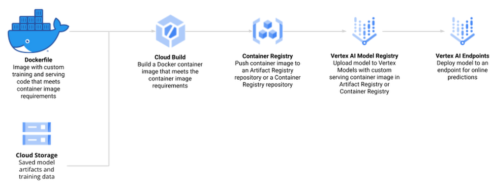
R is one of the most widely used programming languages for statistical computing and machine learning. Many data scientists love it, especially for the rich world of packages from tidyverse, an opinionated collection of R packages for data science. Besides the tidyverse, there are over 18,000 open-source packages on CRAN, the package repository for R. RStudio, available as desktop version or on theGoogle Cloud Marketplace, is a popular Integrated Development Environment (IDE) used by data professionals for visualization and machine learning model development.Once a model has been built successfully, a recurring question among data scientists is: “How do I deploy models written in the R language to production in a scalable, reliable and low-maintenance way?”In this blog post, you will walk through how to use Google Vertex AI to train and deploy  enterprise-grade machine learning models built with R. OverviewManaging machine learning models on Vertex AI can be done in a variety of ways, including using the User Interface of the Google Cloud Console, API calls, or the Vertex AI SDK for Python. Since many R users prefer to interact with Vertex AI from RStudio programmatically, you will interact with Vertex AI through the Vertex AI SDK via the reticulate package. Vertex AI provides pre-built Docker containers for model training and serving predictions for models written in tensorflow, scikit-learn and xgboost. For R, you build a container yourself, derived from Google Cloud Deep Learning Containers for R.Models on Vertex AI can be created in two ways:Train a model locally and import it as a custom model into Vertex AI Model Registry, from where it can be deployed to an endpoint for serving predictions.Create a TrainingPipeline that runs a CustomJob and imports the resulting artifacts as a Model.In this blog post, you will use the second method and train a model directly in Vertex AI since this allows us to automate the model creation process at a later stage while also supporting distributed hyperparameter optimization.The process of creating and managing R models in Vertex AI comprises the following steps:Enable Google Cloud Platform (GCP) APIs and set up the local environmentCreate custom R scripts for training and servingCreate a Docker container that supports training and serving R models with Cloud Build and Container Registry Train a model using Vertex AI Training and upload the artifact to Google Cloud StorageCreate a model endpoint on Vertex AI Prediction Endpoint and deploy the model to serve online prediction requestsMake online predictionFig 1.0 (source)DatasetTo showcase this process, you train a simple Random Forest model to predict housing prices on the California housing data set. The data contains information from the 1990 California census. The data set is publicly available from Google Cloud Storage at gs://cloud-samples-data/ai-platform-unified/datasets/tabular/california-housing-tabular-regression.csvThe Random Forest regressor model will predict a median housing price, given a longitude and latitude along with data from the corresponding census block group. A block group is the smallest geographical unit for which the U.S. Census Bureau publishes sample data (a block group typically has a population of 600 to 3,000 people).Environment SetupThis blog post assumes that you are either using Vertex AI Workbench with an R kernel or RStudio. Your environment should include the following requirements:The Google Cloud SDKGitRPython 3VirtualenvTo execute shell commands, define a helper function:code_block[StructValue([(u’code’, u’library(glue)rnlibrary(IRdisplay)rnrnsh <- function(cmd, args = c(), intern = FALSE) {rn if (is.null(args)) {rn cmd <- glue(cmd)rn s <- strsplit(cmd, ” “)[[1]]rn cmd <- s[1]rn args <- s[2:length(s)]rn }rn ret <- system2(cmd, args, stdout = TRUE, stderr = TRUE)rn if (“errmsg” %in% attributes(attributes(ret))$names) cat(attr(ret, “errmsg”), “n”)rn if (intern) return(ret) else cat(paste(ret, collapse = “n”))rn}’), (u’language’, u”), (u’caption’, <wagtail.wagtailcore.rich_text.RichText object at 0x3eadaafa0290>)])]You should also install a few R packages and update the SDK for Vertex AI:code_block[StructValue([(u’code’, u’install.packages(c(“reticulate”, “glue”))rnsh(“pip install –upgrade google-cloud-aiplatform”)’), (u’language’, u”), (u’caption’, <wagtail.wagtailcore.rich_text.RichText object at 0x3ead93a419d0>)])]Next, you define variables to support the training and deployment process, namely:PROJECT_ID: Your Google Cloud Platform Project IDREGION: Currently, the regions us-central1, europe-west4, and asia-east1 are supported for Vertex AI; it is recommended that you choose the region closest to youBUCKET_URI: The staging bucket where all the data associated with your dataset and model resources are storedDOCKER_REPO: The Docker repository name to store container artifactsIMAGE_NAME: The name of the container imageIMAGE_TAG: The image tag that Vertex AI will useIMAGE_URI: The complete URI of the container imagecode_block[StructValue([(u’code’, u’PROJECT_ID <- “YOUR_PROJECT_ID”rnREGION <- “us-central1″rnBUCKET_URI <- glue(“gs://{PROJECT_ID}-vertex-r”)rnDOCKER_REPO <- “vertex-r”rnIMAGE_NAME <- “vertex-r”rnIMAGE_TAG <- “latest”rnIMAGE_URI <- glue(“{REGION}-docker.pkg.dev/{PROJECT_ID}/{DOCKER_REPO}/{IMAGE_NAME}:{IMAGE_TAG}”)’), (u’language’, u”), (u’caption’, <wagtail.wagtailcore.rich_text.RichText object at 0x3ead93a41550>)])]When you initialize the Vertex AI SDK for Python, you specify a Cloud Storage staging bucket. The staging bucket is where all the data associated with your dataset and model resources are retained across sessions.code_block[StructValue([(u’code’, u’sh(“gsutil mb -l {REGION} -p {PROJECT_ID} {BUCKET_URI}”)’), (u’language’, u”), (u’caption’, <wagtail.wagtailcore.rich_text.RichText object at 0x3ead93a41d90>)])]Next, you import and initialize the reticulate R package to interface with the Vertex AI SDK, which is written in Python.code_block[StructValue([(u’code’, u’library(reticulate)rnlibrary(glue)rnuse_python(Sys.which(“python3″))rnrnaiplatform <- import(“google.cloud.aiplatform”)rnaiplatform$init(project = PROJECT_ID, location = REGION, staging_bucket = BUCKET_URI)’), (u’language’, u”), (u’caption’, <wagtail.wagtailcore.rich_text.RichText object at 0x3ead93a41410>)])]Create Docker container image for training and serving R modelsThe docker file for your custom container is built on top of the Deep Learning container — the same container that is also used for Vertex AI Workbench. In addition, you add two R scripts for model training and serving, respectively.Before creating such a container, you enable Artifact Registry and configure Docker to authenticate requests to it in your region.code_block[StructValue([(u’code’, u’sh(“gcloud artifacts repositories create {DOCKER_REPO} –repository-format=docker –location={REGION} –description=”Docker repository””)rnsh(“gcloud auth configure-docker {REGION}-docker.pkg.dev –quiet”)’), (u’language’, u”), (u’caption’, <wagtail.wagtailcore.rich_text.RichText object at 0x3ead93a41d50>)])]Next, create a Dockerfile.code_block[StructValue([(u’code’, u’# filename: Dockerfile – container specifications for using R in Vertex AIrnFROM gcr.io/deeplearning-platform-release/r-cpu.4-1:latestrnrnWORKDIR /rootrnrnCOPY train.R /root/train.RrnCOPY serve.R /root/serve.Rrnrn# Install FortranrnRUN apt-get updaternRUN apt-get install gfortran -yyrnrn# Install R packagesrnRUN Rscript -e “install.packages(‘plumber’)”rnRUN Rscript -e “install.packages(‘randomForest’)”rnrnEXPOSE 8080′), (u’language’, u”), (u’caption’, <wagtail.wagtailcore.rich_text.RichText object at 0x3ead93a41450>)])]Next, create the file train.R, which is used to train your R model. The script trains a randomForest model on the California Housing dataset. Vertex AI sets environment variables that you can utilize, and since this script uses a Vertex AI managed dataset, data splits are performed by Vertex AI and the script receives environment variables pointing to the training, test, and validation sets. The trained model artifacts are then stored in your Cloud Storage bucket.code_block[StructValue([(u’code’, u’#!/usr/bin/env Rscriptrn# filename: train.R – train a Random Forest model on Vertex AI Managed Datasetrnlibrary(tidyverse)rnlibrary(data.table)rnlibrary(randomForest)rnSys.getenv()rnrn# The GCP Project IDrnproject_id <- Sys.getenv(“CLOUD_ML_PROJECT_ID”)rnrn# The GCP Regionrnlocation <- Sys.getenv(“CLOUD_ML_REGION”)rnrn# The Cloud Storage URI to upload the trained model artifact tornmodel_dir <- Sys.getenv(“AIP_MODEL_DIR”)rnrn# Next, you create directories to download our training, validation, and test set into.rndir.create(“training”)rndir.create(“validation”)rndir.create(“test”)rnrn# You download the Vertex AI managed data sets into the container environment locally.rnsystem2(“gsutil”, c(“cp”, Sys.getenv(“AIP_TRAINING_DATA_URI”), “training/”))rnsystem2(“gsutil”, c(“cp”, Sys.getenv(“AIP_VALIDATION_DATA_URI”), “validation/”))rnsystem2(“gsutil”, c(“cp”, Sys.getenv(“AIP_TEST_DATA_URI”), “test/”))rnrn# For each data set, you may receive one or more CSV files that you will read into data frames.rntraining_df <- list.files(“training”, full.names = TRUE) %>% map_df(~fread(.))rnvalidation_df <- list.files(“validation”, full.names = TRUE) %>% map_df(~fread(.))rntest_df <- list.files(“test”, full.names = TRUE) %>% map_df(~fread(.))rnrnprint(“Starting Model Training”)rnrf <- randomForest(median_house_value ~ ., data=training_df, ntree=100)rnrfrnrnsaveRDS(rf, “rf.rds”)rnsystem2(“gsutil”, c(“cp”, “rf.rds”, model_dir))’), (u’language’, u”), (u’caption’, <wagtail.wagtailcore.rich_text.RichText object at 0x3ead920dc110>)])]Next, create the file serve.R, which is used for serving your R model. The script downloads the model artifact from Cloud Storage, loads the model artifacts, and listens for prediction requests on port 8080. You have several environment variables for the prediction service at your disposal, including:AIP_HEALTH_ROUTE: HTTP path on the container that AI Platform Prediction sends health checks to.AIP_PREDICT_ROUTE: HTTP path on the container that AI Platform Prediction forwards prediction requests to.code_block[StructValue([(u’code’, u’#!/usr/bin/env Rscriptrn# filename: serve.R – serve predictions from a Random Forest modelrnSys.getenv()rnlibrary(plumber)rnrnsystem2(“gsutil”, c(“cp”, “-r”, Sys.getenv(“AIP_STORAGE_URI”), “.”))rnsystem(“du -a .”)rnrnrf <- readRDS(“artifacts/rf.rds”)rnlibrary(randomForest)rnrnpredict_route <- function(req, res) {rn print(“Handling prediction request”)rn df <- as.data.frame(req$body$instances)rn preds <- predict(rf, df)rn return(list(predictions=preds))rn}rnrnprint(“Staring Serving”)rnrnpr() %>%rn pr_get(Sys.getenv(“AIP_HEALTH_ROUTE”), function() “OK”) %>%rn pr_post(Sys.getenv(“AIP_PREDICT_ROUTE”), predict_route) %>%rn pr_run(host = “0.0.0.0”, port=as.integer(Sys.getenv(“AIP_HTTP_PORT”, 8080)))’), (u’language’, u”), (u’caption’, <wagtail.wagtailcore.rich_text.RichText object at 0x3ead920dcf10>)])]Next, you build the Docker container image on Cloud Build — the serverless CI/CD platform.  Building the Docker container image may take 10 to 15 minutes.code_block[StructValue([(u’code’, u’sh(“gcloud builds submit –region={REGION} –tag={IMAGE_URI} –timeout=1h”)’), (u’language’, u”), (u’caption’, <wagtail.wagtailcore.rich_text.RichText object at 0x3ead920dcc90>)])]Create Vertex AI Managed DatasetYou create a Vertex AI Managed Dataset to have Vertex AI take care of the data set split. This is optional, and alternatively you may want to pass the URI to the data set via environment variables.code_block[StructValue([(u’code’, u’data_uri <- “gs://cloud-samples-data/ai-platform-unified/datasets/tabular/california-housing-tabular-regression.csv”rnrndataset <- aiplatform$TabularDataset$create(rn display_name = “California Housing Dataset”,rn gcs_source = data_urirn)’), (u’language’, u”), (u’caption’, <wagtail.wagtailcore.rich_text.RichText object at 0x3ead920dc650>)])]The next screenshot shows the newly created Vertex AI Managed dataset in Cloud Console.Train R Model on Vertex AIThe custom training job wraps the training process by creating an instance of your container image and executing train.R for model training and serve.R for model serving.Note: You use the same custom container for both training and serving.code_block[StructValue([(u’code’, u’job <- aiplatform$CustomContainerTrainingJob(rn display_name = “vertex-r”,rn container_uri = IMAGE_URI,rn command = c(“Rscript”, “train.R”),rn model_serving_container_command = c(“Rscript”, “serve.R”),rn model_serving_container_image_uri = IMAGE_URIrn)’), (u’language’, u”), (u’caption’, <wagtail.wagtailcore.rich_text.RichText object at 0x3ead93040050>)])]To train the model, you call the method run(), with a machine type that is sufficient in resources to train a machine learning model on your dataset. For this tutorial, you use a n1-standard-4 VM instance.code_block[StructValue([(u’code’, u’model <- job$run(rn dataset=dataset,rn model_display_name = “vertex-r-model”,rn machine_type = “n1-standard-4″rn)rnrnmodel$display_namernmodel$resource_namernmodel$uri’), (u’language’, u”), (u’caption’, <wagtail.wagtailcore.rich_text.RichText object at 0x3ead930402d0>)])]The model is now being trained, and you can watch the progress in the Vertex AI Console.Provision an Endpoint resource and deploy a ModelYou create an Endpoint resource using the Endpoint.create() method. At a minimum, you specify the display name for the endpoint. Optionally, you can specify the project and location (region); otherwise the settings are inherited by the values you set when you initialized the Vertex AI SDK with the init() method.In this example, the following parameters are specified:display_name: A human readable name for the Endpoint resource.project: Your project ID.location: Your region.labels: (optional) User defined metadata for the Endpoint in the form of key/value pairs.This method returns an Endpoint object.code_block[StructValue([(u’code’, u’endpoint <- aiplatform$Endpoint$create(rn display_name = “California Housing Endpoint”,rn project = PROJECT_ID,rn location = REGIONrn)’), (u’language’, u”), (u’caption’, <wagtail.wagtailcore.rich_text.RichText object at 0x3ead93040ed0>)])]You can deploy one of more Vertex AI Model resource instances to the same endpoint. Each Vertex AI Model resource that is deployed will have its own deployment container for the serving binary.Next, you deploy the Vertex AI Model resource to a Vertex AI Endpoint resource. The Vertex AI Model resource already has defined for it the deployment container image. To deploy, you specify the following additional configuration settings:The machine type.The (if any) type and number of GPUs.Static, manual or auto-scaling of VM instances.In this example, you deploy the model with the minimal amount of specified parameters, as follows:model: The Model resource.deployed_model_displayed_name: The human readable name for the deployed model instance.machine_type: The machine type for each VM instance.Due to the requirements to provision the resource, this may take up to a few minutes.Note: For this example, you specified the R deployment container in the previous step of uploading the model artifacts to a Vertex AI Model resource.code_block[StructValue([(u’code’, u’model$deploy(endpoint = endpoint, machine_type = “n1-standard-4″)’), (u’language’, u”), (u’caption’, <wagtail.wagtailcore.rich_text.RichText object at 0x3ead93040b50>)])]The model is now being deployed to the endpoint, and you can see the result in the Vertex AI Console.Make predictions using newly created EndpointFinally, you create some example data to test making a prediction request to your deployed model. You use five JSON-encoded example data points (without the label median_house_value) from the original data file in data_uri. Finally, you make a prediction request with your example data. In this example, you use the REST API (e.g., Curl) to make the prediction request.code_block[StructValue([(u’code’, u’library(jsonlite)rndf <- read.csv(text=sh(“gsutil cat {data_uri}”, intern = TRUE))rnhead(df, 5)rnrninstances <- list(instances=head(df[, names(df) != “median_house_value”], 5))rninstancesrnrnjson_instances <- toJSON(instances)rnurl <- glue(“https://{REGION}-aiplatform.googleapis.com/v1/{endpoint$resource_name}:predict”)rnaccess_token <- sh(“gcloud auth print-access-token”, intern = TRUE)rnrnsh(rn “curl”,rn c(“–tr-encoding”,rn “-s”,rn “-X POST”,rn glue(“-H ‘Authorization: Bearer {access_token}'”),rn “-H ‘Content-Type: application/json'”,rn url,rn glue(“-d {json_instances}”)rn ),rn)’), (u’language’, u”), (u’caption’, <wagtail.wagtailcore.rich_text.RichText object at 0x3ead93040b90>)])]The endpoint now returns five predictions in the same order the examples were sent.CleanupTo clean up all Google Cloud resources used in this project, you can delete the Google Cloud project you used for the tutorial or delete the created resources.code_block[StructValue([(u’code’, u’endpoint$undeploy_all()rnendpoint$delete()rndataset$delete()rnmodel$delete()rnjob$delete()’), (u’language’, u”), (u’caption’, <wagtail.wagtailcore.rich_text.RichText object at 0x3ead93078150>)])]SummaryIn this blog post, you have gone through the necessary steps to train and deploy an R model to Vertex AI. For easier reproducibility, you can refer to this Notebook on GitHubAcknowledgementsThis blog post received contributions from various people. In particular, we would like to thank  Rajesh Thallam for strategic and technical oversight, Andrew Ferlitsch for technical guidance, explanations, and code reviews, and Yuriy Babenko for reviews.
Quelle: Google Cloud Platform

No pipelines needed. Stream data with Pub/Sub direct to BigQuery

Pub/Sub’s ingestion of data into BigQuery can be critical to making your latest business data immediately available for analysis. Until today, you had to create intermediate Dataflow jobs before your data could be ingested into BigQuery with the proper schema. While Dataflow pipelines (including ones built with Dataflow Templates) get the job done well, sometimes they can be more than what is needed for use cases that simply require raw data with no transformation to be exported to BigQuery.Starting today, you no longer have to write or run your own pipelines for data ingestion from Pub/Sub into BigQuery. We are introducing a new type of Pub/Sub subscription called a “BigQuery subscription” that writes directly from Cloud Pub/Sub to BigQuery. This new extract, load, and transform (ELT) path will be able to simplify your event-driven architecture. For Pub/Sub messages where advanced preload transformations or data processing before landing data in BigQuery (such as masking PII) is necessary, we still recommend going through Dataflow.Get started by creating a new BigQuery subscription that is associated with a Pub/Sub topic. You will need to designate an existing BigQuery table for this subscription. Note that the table schema must adhere to certain compatibility requirements. By taking advantage of Pub/Sub topic schemas, you have the option of writing Pub/Sub messages to BigQuery tables with compatible schemas. If schema is not enabled for your topic, messages will be written to BigQuery as bytes or strings. After the creation of the BigQuery subscription, messages will now be directly ingested into BigQuery.Better yet, you no longer need to pay for data ingestion into BigQuery when using this new direct method. You only pay for the Pub/Sub you use. Ingestion from Pub/Sub’s BigQuery subscription into BigQuery costs $50/TiB based on read (subscribe throughput) from the subscription. This is a simpler and cheaper billing experience compared to the alternative path via Dataflow pipeline where you would be paying for the Pub/Sub read, Dataflow job, and BigQuery data ingestion. See the pricing page for details. To get started, you can read more about Pub/Sub’s BigQuery subscription or simply create a new BigQuery subscription for a topic using Cloud Console or the gcloud CLI.
Quelle: Google Cloud Platform

70 apps in 2 years: How Renault tackled database migration

Editor’s note: Renault, the French automaker, embarked on a wholesale migration of its information systems—moving 70 applications to Google Cloud. Here’s how they migrated from Oracle databases to Cloud SQL for PostgreSQL.The Renault Group, known for its iconic French cars has grown to include four complementary brands, and sold nearly 3 million vehicles in 2020. Following our company-wide strategic plan, “Renaulution,” we’ve shifted our focus over the past year from a car company integrating tech, to a tech company integrating cars that will develop software for our business. For the information systems group, that meant modernizing our entire portfolio and migrating 70 in-house applications (our quality and customer information systems) to Google Cloud. It was an ambitious project, but it’s paid off. In two years we migrated our Quality and Customer Satisfaction information systems applications, optimized our code, and cut costs thanks to managed database services. Compared to our on-premises infrastructure, using Google Cloud services and open-source technologies comes to roughly one dollar per user per year, which is significantly cheaper. An ambitious journey to Google CloudWe began our cloud journey in 2016 with digital projects integrating a new way of working and new technologies. These new technologies included those for agility at scale, data capabilities and CI/CD toolchain. Google Cloud stood out as the clear choice for its data capabilities. Not only are we using BigQuery and Dataflow to improve scaling and costs, but we are also now using fully managed database services like Cloud SQL for PostgreSQL. Data is a key asset for a modern car maker because it connects the car maker to the user, allows car makers to better understand usage and better informs what decisions we should make about our products and services. After we migrated our data lake to Google Cloud, it was a natural next step to move our front-end applications to Google Cloud so they would be easier to maintain and we could benefit from faster response times. This project was no small undertaking. For those 70 in-house applications (e.g. vehicle quality evaluation, statistical process control in plants, product issue management, survey analysis) for our information systems landscape, we had a range of technologies—including Oracle, MySQL, Java, IBM MQ, and CFT—with some applications created 20 years ago. Champions spearhead each migrationBefore we started the migration, we did a global analysis of the landscape to understand each application and its complexity. Then we planned a progressive approach, focusing on the smallest applications first such as those with a limited number of screens or with simple SQL queries, and saving the largest for last. Initially we used some automatic tools for the migration, but we learned very quickly nothing can replace the development team’s institutional knowledge. They served as our migration champions.The apps go marching one by oneWhen we migrated our first few Oracle databases to Cloud SQL for PostgreSQL we tracked our learnings in an internal wiki to share common SQL patterns, which helped us speed up the process. For some applications, we simplified the architecture and took the opportunity to analyze and optimize SQL queries during the rework. We also used monitoring tools like Dynatrace and JavaMelody to ensure we improved the user experience.The approach we developed was very successful—where database migration was initially seen as insurmountable, the entire migration project was completed in two years.With on-premises applications it was hard for our developers to separate code performance from infrastructure limitations. So as part of our migration to Google Cloud, we optimized our applications with monitoring services. With these insights our team has more control over resources, which has reduced our maintenance and operations activity and resulted in faster, more stable applications. Plus, migrating to Cloud SQL has made it much easier for us to change our infrastructure as needed, add more power when necessary or even reduce our infrastructure size. A new regime on Cloud SQLNow that we’re running on Cloud SQL, we’ve improved performance even on large databases with many connected users. Thanks to built-in tools in the Google Cloud environment, we can now easily understand performance issues and quickly solve them. For example, we were able to reduce the duration of a heavy batch processing by a factor of three from nine to three hours. And we don’t have to wait for the installation of a new server, so our team can move faster. Beyond speed, we’ve also been able to cut costs. We optimized our code based on insights from monitoring tools, which not only enabled a more responsive application for the user, but it also reduced our costs because we’re not overprovisioned.   Learn more about the Renault Group and try out Cloud SQL today.Related ArticleHow Kitabisa re-structured its fundraising platform to drive “kindness at scale” on Google CloudThe Indonesian fundraising platform overhauled its platform by moving to containers, a microservices architecture and Cloud SQL and Proxy…Read Article
Quelle: Google Cloud Platform