Cloud Wisdom Weekly: 5 ways to reduce costs with containers

“Cloud Wisdom Weekly: for tech companies and startups” is a new blog series we’re running this fall to answer common questions our tech and startup customers ask us about how to build apps faster, smarter, and cheaper. In this installment, Google Cloud Product Manager Rachel Tsao explores how to save on compute costs with modern container platforms. Many tech companies and startups are built to operate under a certain degree of pressure and to efficiently manage costs and resources. These pressures have only increased with inflation, geopolitical shifts, and supply chain concerns, however, creating urgency for companies to find ways to preserve capital while increasing flexibility. The right approach to containers can be crucial to navigating these challenges. In the last few years, development teams have shifted from virtual machines (VMs) to containers, drawn to the latter because they are faster, more lightweight, and easier to manage and automate. Containers also consume fewer resources than VMs, by leveraging shared operating systems. Perhaps most importantly, containers enable portability, letting developers put an application and all its dependencies into a single package that can run almost anywhere. Containers are central to an organization’s agility, and in our conversations with customers about why they choose Google Cloud, we hear frequently that services like Google Kubernetes Engine (GKE) and Cloud Run help tech companies and startups to not only go to market quickly, but also save money. In this article, we’ll explore five ways to help your business quickly and easily reduce compute costs with containers. 5 ways to control compute costs with containers Whether your company is  an established player that is modernizing its business or a startup building its first product, managed containerized products can help you reduce costs, optimize development, and innovate. The following tips will help you to evaluate core features you should expect of container services and include specific advice for GKE and Cloud Run.1. Identify opportunities to reduce cluster administration Most companies want to dedicate resources to innovation, not infrastructure curation. If your team has existing Kubernetes knowledge or runs workloads that need to leverage machine types or graphics processing units (GPUs), you may be able to simplify provisioning with GKE Autopilot. GKE Autopilot provisions and manages the cluster’s underlying infrastructure, all while you pay for only the workload, not 24/7 access to the underlying node-pool compute VMs. In this way, it can reduce cluster administration while saving you money and giving you hardened security best practices by default.2. Consider serverless to maximize developer productivity Serverless platforms continue the theme of empowering your technical talent to focus on the most impactful work. Such platforms can promote productivity by abstracting away aspects of infrastructure creation, letting developers work on projects that drive the business while the platform provider oversees hardware and scalability, aspects of security, and more.  For a broad range of workloads that don’t need machine types or GPUs, going serverless with Cloud Run is a great option for building applications, APIs, internal services, and even real-time data pipelines. Analyst research supports that Cloud Run customers achieve faster deployments with less time spent monitoring services, resulting in reinvested productivity that lets these customers do more with fewer resources.  Designed with high scalability in mind, and an emphasis on the portability of containers, Cloud Run also supports a wide range of stateless workloads, including jobs that run to completion. Moreover, it lets you maximize the skills of your existing team, as it does not require cluster management, a Kubernetes skillset or prior infrastructure experience. Additionally, Cloud Run leverages the Knative spec and a container image as a deployment artifact, enabling an easy migration to GKE if your workload needs change.With Cloud Run, gone are the days of infrastructure overprovisioning! The platform scales down to zero automatically, meaning your services always have the capacity to meet demand, but do not incur costs if there is no traffic. 3. Save with committed use discountsCommitted use discounts provide discounted pricing in exchange for committing to a minimal level of usage in a region for a specified term. If you are able to reliably predict your resource needs, for instance, you can get a 17% discount for Cloud Run (for either one year or three years), and either a 20% discount (for one year) or a 45% discount (for three years) on GKE Autopilot.4. Leverage cost management features Minimum and maximum instances are useful for ensuring your services are ready to receive requests but do not cause cost overages. For Google Cloud customers, best practices for cost management include building your container with Cloud Build, which offers pay-for-use pricing and can be more cost efficient than steady-state build farms.Relatedly, if you choose to leverage serverless containers with Cloud Run, you can set minimum instances to avoid the lag (i.e., the cold start) when a new container instance is starting up from zero. Minimum instances are billed at one-tenth of the general Cloud Run cost. Likewise, if you are testing and want to avoid costs spiraling, you can set a maximum number of instances to ensure your containers do not scale beyond a certain threshold. These settings can be turned off anytime, resulting in no costs when your service is not processing traffic. To have better oversight of costs, you can also view built-in billing reports and set budget alerts on Cloud Billing. 5. Match workload needs to pricing modelsGKE Autopilot is great for running highly reliable workloads thanks to its Pod-level SLA. But if you have workloads that do not need a high level of reliability (e.g., fault tolerant batch workloads, dev/test clusters), you can leverage spot pricing to receive a discount of 60% to 91% compared to regularly-priced pods. Spot Pods run on spare Google Cloud compute capacity as long as resources are available. GKE will evict your Spot Pod with a grace period of 25 seconds during times of high resource demand, but you can automatically redeploy as soon as there is available capability. This can result in significant savings for workloads that are a fit. Innovation requires balance Put into practice, these tips can help you and your business to get the most out of containers while controlling management and resource costs. That said, it is worth noting that while managing cloud costs is important, the relationship between “cloud” and “cost” is often complex. If you are adopting cloud computing with only the primary goal of saving money, you may soon run into other challenges. Cloud services can save your business money in many ways, but they can also help you get the most value for your money. This balance between cost efficiency and absolute cost is important to keep in mind so that even in challenging economic landscapes, your tech company or startup can continue growing and innovating. Beyond cost savings, many tech and startup companies are seeking improved business agility, which is the ability to deploy new products and features frequently and with high quality. With deployment best practices built into GKE Autopilot and Cloud Run, you can transform the way your team operates while maximizing productivity with every new deployment. You can learn if your existing workloads are appropriate for containers with this fit assessment and these guides for migrating to containers. For new workloads, you can leverage these guides for GKE Autopilot and Cloud Run. And for more tips on cost optimization, check out our Architecture Framework for compute, containers, and serverless.If you want to learn more about how Google Cloud can help your startup, visit our page here to get more information about our program and apply for our Google for Startups Cloud Program, and sign up for our communications to get a look at our community activities, digital events, special offers, and more.Related ArticleThink serverless: tips for early-stage startupsGoogle Cloud tips for early-stage startups, from leveraging serverless to maximizing cloud credits to comparing managed services.Read Article
Quelle: Google Cloud Platform

Integrating ML models into production pipelines with Dataflow

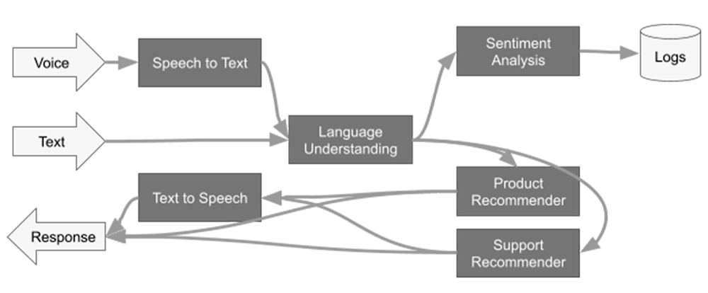
Google Cloud’s Dataflow recently announced the General Availability support for Apache Beam’s generic machine learning prediction and inference transform, RunInference. In this blog, we will take a deeper dive on the transform, including:Showing the RunInference transform used with a simple model as an example, in both batch and streaming mode.Using the transform with multiple models in an ensemble.Providing an end-to-end pipeline example that makes use of an open source model from Torchvision. In the past, Apache Beam developers who wanted to make use of a machine learning model locally, in a production pipeline, had to hand-code the call to the model within a user defined function (DoFn), taking on the technical debt for layers of boilerplate code. Let’s have a look at what would have been needed:Load the model from a common location using the framework’s load method.Ensure that the model is shared amongst the DoFns, either by hand or via the shared class utility in Beam.Batch the data before the model is invoked to improve the model efficiency. The developer would set this up, either by hand or via one of the groups into batches utilities.Provide a set of metrics from the transform.Provide production grade logging and exception handling with clean messages to help that SRE out at 2 in the morning! Pass specific parameters to the models, or start to build a generic transform that allows the configuration to determine information within the model. And of course these days, companies need to deploy many models, so the data engineer begins to do what all good data engineers do and builds out an abstraction for the models. Basically, each company is building out their own RunInference transform!  Recognizing that all of this activity is mostly boilerplate regardless of the model, the RunInference API was created. The inspiration for this API comes from the tfx_bsl.RunInference transform that the good folks over at TensorFlow Extended built to help with exactly the issues described above. tfx_bsl.RunInference was built around TensorFlow models. The new Apache Beam RunInference transform is designed to be framework agnostic and easily composable in the Beam pipeline. The signature for RunInference takes the form of RunInference(model_handler), where the framework-specific configuration and implementation is dealt with in the model_handler configuration object. This creates a clean developer experience and allows for new frameworks to be easily supported within the production machine learning pipeline, without disrupting the developer workflow.. For example, NVIDIA is contributing to the Apache Beam project to integrateNVIDIA TensorRTTM, an SDK that can optimize trained models for deployment with the highest throughput and lowest latency on NVIDIA GPUs within Google Dataflow (PullRequest).  Beam Inference also allows developers to make full use of the versatility of Apache Beam’s pipeline model, making it easier to build complex multi-model pipelines with minimum effort. Multi-model pipelines are useful for activities like A/B testing and building out ensembles. For example, doing natural language processing (NLP) analysis of text and then using the results within a domain specific model to drive a customer recommendation. In the next section, we start to explore the API using code from the public codelab with the notebook also available at github.com/apache/beam/examples/notebooks/beam-ml.Using the Beam Inference APIBefore we get into the API, for those who are unfamiliar with Apache Beam, let’s put together a small pipeline that reads data from some CSV files to get us warmed up on the syntax.code_block[StructValue([(u’code’, u”import apache_beam as beamrnrnwith beam.Pipeline() as p:rn data = p | beam.io.ReadFromText(‘./file.csv’) rn data | beam.Map(print)”), (u’language’, u”), (u’caption’, <wagtail.wagtailcore.rich_text.RichText object at 0x3eaaa26ab6d0>)])]In that pipeline, we used the ReadFromText source to consume the data from the CSV file into a Parallel Collection, referred to as a PCollection in Apache Beam. In Apache Beam syntax, the pipe ‘|’ operator essentially means “apply”, so the first line applies the ReadFromText transform. In the next line, we use a beam.Map() to do element-wise processing of the data; in this case, the data is just being sent to the print function.Next, we make use of a very simple model to show how we can configure RunInference with different frameworks. The model is a single-layer linear regression that has been trained on y = 5x data (yup, it’s learned its fives times table). To build this model, follow the steps in the codelab. The RunInference transform has the following signature: RunInference(ModelHandler). The ModelHandler is a configuration that informs RunInference about the model details and that provides type information for the output. In the codelab, the PyTorch saved model file is named ‘five_times_table_torch.pt’ and is output as a result of the call to torch.save() on the model’s state_dict. Let’s create a ModelHandler that we can pass to RunInference for this model:code_block[StructValue([(u’code’, u”my_handler = PytorchModelHandlerTensor(rn state_dict_path=./five_times_table_torch.pt,rn model_class=LinearRegression,rn model_params={‘input_dim': 1,rn ‘output_dim': 1}”), (u’language’, u”), (u’caption’, <wagtail.wagtailcore.rich_text.RichText object at 0x3eaa926196d0>)])]The model_class is the class of the PyTorch model that defines the model architecture as a subclass of torch.nn.Module. The model_params are the ones that are defined by the constructor of the model_class. In this example, they are used in the notebook LinearRegression class definition:code_block[StructValue([(u’code’, u’class LinearRegression(torch.nn.Module):rn def __init__(self, input_dim=1, output_dim=1):rn super().__init__()rn self.linear = torch.nn.Linear(input_dim, output_dim) rn def forward(self, x):rn out = self.linear(x)rn return out’), (u’language’, u”), (u’caption’, <wagtail.wagtailcore.rich_text.RichText object at 0x3eaaa25e92d0>)])]The ModelHandler that is used also provides the transform information about the input type to the model, with PytorchModelHandlerTensor expecting torch.Tensor elements.To make use of this configuration, we update our pipeline with the configuration. We will also do the pre-processing needed to get the data into the right shape and type for the model that has been created. The model expects a torch.Tensor of shape [-1,1] and the data in our CSV file is in the format 20,30,40.code_block[StructValue([(u’code’, u”with beam.Pipeline() as p:rn raw_data = p | beam.io.ReadFromText(‘./file.csv’)rn shaped_data = raw_data | beam.FlatMap(lambda x : rn [numpy.float32(y).reshape(-1,1) rn for y in x.split(‘,’)]))rn results = shaped_data | beam.Map(torch.Tensor) | RunInference(my_handler)rn results | beam.Map(print)”), (u’language’, u”), (u’caption’, <wagtail.wagtailcore.rich_text.RichText object at 0x3eaa91962f50>)])]This pipeline will read the CSV file, get the data into shape for the model, and run the inference for us. The result of the print statement can be seen here:PredictionResult(example=tensor([20.]), inference=tensor([100.0047], grad_fn=<UnbindBackward0>))The PredictionResult object contains both the example as well as the result, in this case 100.0047 given an input of 20. Next, we look at how composing multiple RunInference transforms within a single pipeline gives us the ability to build out complex ensembles with a few lines of code. After that, we will look at a real model example with TorchVision.Multi model pipelinesIn the previous example, we had one model, a source, and an output. That pattern will be used by many pipelines. However, business needs also require ensembles of models where models are used for pre-processing of the data and for the domain specific tasks. For example, conversion of speech to text before being passed to an NLP model. Though the diagram above is a complex flow, there are actually three primary patterns. 1- Data is flowing down the graph.2- Data can branch after a stage, for example after ‘Language Understanding’.3- Data can flow from one model into another.Item 1 means that this is a good fit for building into a single Beam pipeline because it’s acyclic. For items 2 and 3, the Beam SDK can express the code very simply. Let’s take a look at these.Branching Pattern:In this pattern, data is branched to two models. To send all the data to both models, the code is in the form:code_block[StructValue([(u’code’, u’model_a_predictions = shaped_data | RunInference(configuration_model_a)rn model_b_predictions = shaped_data | RunInference(configuration_model_b)’), (u’language’, u”), (u’caption’, <wagtail.wagtailcore.rich_text.RichText object at 0x3eaaa2307890>)])]Models in Sequence:In this pattern, the output of the first model is sent to the next model. Some form of post processing normally occurs between these stages. To get the data in the right shape for the next step, the code is in the form:code_block[StructValue([(u’code’, u’model_a_predictions = shaped_data | RunInference(configuration_model_a)rnmodel_b_predictions = (model_a_predictions | beam.Map(postprocess) rn | RunInference(configuration_model_b))’), (u’language’, u”), (u’caption’, <wagtail.wagtailcore.rich_text.RichText object at 0x3eaaa031ff50>)])]With those two simple patterns (branching and model in sequence) as building blocks, we see that it’s possible to build complex ensembles of models. You can also make use of other Apache Beam tools to enrich the data at various stages in these pipelines. For example, in a sequential model, you may want to join the output of model a with data from a database before passing it to model b, bread and butter work for Beam. Using an open source modelIn the first example, we used a toy model that was available in the codelab. In this section, we walk through how you could use an open source model and output the model data to a Data Warehouse (Google Cloud BigQuery) to show a more complete end-to-end pipeline.Note that the code in this section is self-contained and not part of the codelab used in the previous section. The PyTorch model we will use to demonstrate this is maskrcnn_resnet50_fpn, which comes with Torchvision v 0.12.0. This model attempts to solve the image segmentation task: given an image, it detects and delineates each distinct object appearing in that image with a bounding box.In general, libraries like Torchvision pretrained models download the pretrained model directly into memory. To run the model with RunInference, we need a different setup, because RunInference will load the model once per Python process to be shared amongst many threads. So if we want to use a pre-trained model from these types of libraries, we have a little bit of setup to do. For this PyTorch model we need to:1- Download the state dictionary and make it available independently of the library to Beam.2- Determine the model class file and provide it to our ModelHandler, ensuring that we disable the class’s ‘autoload’ features.When looking at the signature for this model with version 0.12.0, note that there are two parameters that initiate an auto-download: pretrained and pretrained_backbone. Ensure these are both set to False to make sure that the model class does not load the model files:model_params = {‘pretrained': False, ‘pretrained_backbone': False}Step 1 – Download the state dictionary. The location can be found in the maskrcnn_resnet50_fpn source code:code_block[StructValue([(u’code’, u’%pip install apache-beam[gcp] torch==1.11.0 torchvision==0.12.0′), (u’language’, u”), (u’caption’, <wagtail.wagtailcore.rich_text.RichText object at 0x3eaaa2873c10>)])]code_block[StructValue([(u’code’, u’import os,iornfrom PIL import Imagernfrom typing import Tuple, Anyrnimport torch, torchvisionrnimport apache_beam as beamrnfrom apache_beam.io import fileiornfrom apache_beam.io.gcp.internal.clients import bigqueryrnfrom apache_beam.options.pipeline_options import PipelineOptionsrnfrom apache_beam.options.pipeline_options import SetupOptionsrnfrom apache_beam.ml.inference.base import KeyedModelHandlerrnfrom apache_beam.ml.inference.base import PredictionResultrnfrom apache_beam.ml.inference.pytorch_inference import PytorchModelHandlerTensor’), (u’language’, u”), (u’caption’, <wagtail.wagtailcore.rich_text.RichText object at 0x3eaaa2873d10>)])]code_block[StructValue([(u’code’, u”# Download the state_dict using the torch hub utility to a local models directoryrntorch.hub.load_state_dict_from_url(‘https://download.pytorch.org/models/maskrcnn_resnet50_fpn_coco-bf2d0c1e.pth’, ‘models/’)”), (u’language’, u”), (u’caption’, <wagtail.wagtailcore.rich_text.RichText object at 0x3eaa9371a9d0>)])]Next, push this model from the local directory where it was downloaded to a common area accessible to workers. You can use utilities like gsutil if using Google Cloud Storage (GCS) as your object store:code_block[StructValue([(u’code’, u”model_path = f’gs://{bucket}/models/maskrcnn_resnet50_fpn_coco-bf2d0c1e.pth'”), (u’language’, u”), (u’caption’, <wagtail.wagtailcore.rich_text.RichText object at 0x3eaa916f93d0>)])]Step 2 – For our Modelandler, we need to use the model_class, which in our case is torchvision.models.detection.maskrcnn_resnet50_fpn. We can now build our ModelHandler. Note that in this case, we are making a KeyedModelHandler, which is different from the simple example we used above. The KeyedModelHandler is used to indicate that the values coming into the RunInference API are a tuple, where the first value is a key and the second is the tensor that will be used by the model. This allows us to keep a reference of which image the inference is associated with, and it is used in our post processing step.code_block[StructValue([(u’code’, u”my_cloud_model_handler = PytorchModelHandlerTensor(rn state_dict_path=model_path,rn model_class=torchvision.models.detection.maskrcnn_resnet50_fpn,rn model_params={‘pretrained':False, ‘pretrained_backbone’ : False})rnrnmy_keyed_cloud_model_handler = KeyedModelHandler(my_cloud_model_handler)”), (u’language’, u”), (u’caption’, <wagtail.wagtailcore.rich_text.RichText object at 0x3eaa916f9990>)])]All models need some level of pre-processing. Here we create a preprocessing function ready for our pipeline. One important note: when batching, the PyTorch ModelHandler will need the size of the tensor to be the same across the batch, so here we set the image_size as part of the pre-processing step. Also note that this function accepts a tuple with the first element being a string. This will be the ‘key’, and in the pipeline code, we will use the filename as the key.code_block[StructValue([(u’code’, u’# In this function we can carry out any pre-processing steps that you need for the modelrnrndef preprocess_image(data: Tuple[str,Image.Image]) -> Tuple[str,torch.Tensor]:rn import torchrn import torchvision.transforms as transformsrn # Note RunInference will by default auto batch inputs for Torch modelsrn # Alternative to this is to create a wrapper class, and overriding the batch_elements_kwargsrn # function to return {max_batch_size=1}set max_batch_size=1rn image_size = (224, 224)rn transform = transforms.Compose([rn transforms.Resize(image_size),rn transforms.ToTensor(),rn ])rn return data[0], transform(data[1])’), (u’language’, u”), (u’caption’, <wagtail.wagtailcore.rich_text.RichText object at 0x3eaa916f9310>)])]The output of the model needs some post processing before being sent to BigQuery. Here we denormalise the label with the actual name, for example, person, and zip it up with the bounding box and score output:code_block[StructValue([(u’code’, u”# The inference result is a PredictionResult object, this has two components the example and the inferencerndef post_process(kv : Tuple[str, PredictionResult]):rn # We will need the coco labels to translate the output from the modelrn coco_names = [‘unlabeled’, ‘person’, ‘bicycle’, ‘car’, ‘motorcycle’,rn ‘airplane’, ‘bus’, ‘train’, ‘truck’, ‘boat’, ‘traffic light’,rn ‘fire hydrant’, ‘street sign’, ‘stop sign’, ‘parking meter’,rn ‘bench’, ‘bird’, ‘cat’, ‘dog’, ‘horse’, ‘sheep’, ‘cow’,rn ‘elephant’, ‘bear’, ‘zebra’, ‘giraffe’, ‘hat’, ‘backpack’,rn ‘umbrella’, ‘shoe’, ‘eye glasses’, ‘handbag’, ‘tie’, ‘suitcase’,rn ‘frisbee’, ‘skis’, ‘snowboard’, ‘sports ball’, ‘kite’,rn ‘baseball bat’, ‘baseball glove’, ‘skateboard’, ‘surfboard’,rn ‘tennis racket’, ‘bottle’, ‘plate’, ‘wine glass’, ‘cup’, ‘fork’,rn ‘knife’, ‘spoon’, ‘bowl’, ‘banana’, ‘apple’, ‘sandwich’,rn ‘orange’, ‘broccoli’, ‘carrot’, ‘hot dog’, ‘pizza’, ‘donut’,rn ‘cake’, ‘chair’, ‘couch’, ‘potted plant’, ‘bed’, ‘mirror’,rn ‘dining table’, ‘window’, ‘desk’, ‘toilet’, ‘door’, ‘tv’,rn ‘laptop’, ‘mouse’, ‘remote’, ‘keyboard’, ‘cell phone’,rn ‘microwave’, ‘oven’, ‘toaster’, ‘sink’, ‘refrigerator’,rn ‘blender’, ‘book’, ‘clock’, ‘vase’, ‘scissors’, ‘teddy bear’,rn ‘hair drier’, ‘toothbrush’]rn # Extract the outputrn output = kv[1].inferencern # The model outputs labels, boxes and scores, we pull these out and creatern # a tuple with the label mapped to the coco_names and convert the tensorsrn return {‘file’ : kv[0], ‘inference’ : [rn {‘label': coco_names[x],rn ‘box’ : y.detach().numpy().tolist(),rn ‘score’ : z.item()}rn for x,y,z in zip(output[‘labels’],rn output[‘boxes’],rn output[‘scores’])]}”), (u’language’, u”), (u’caption’, <wagtail.wagtailcore.rich_text.RichText object at 0x3eaaa424bb50>)])]Let’s now run this pipeline with the direct runner, which will read the image from GCS, run it through the model, and output the results to BigQuery. We will need to pass in the BigQuery schema that we want to use, which should match the dict that we created in our post-processing. The WriteToBigquery transform takes the schema information as the table_spec object, which represents the following schema:The schema has a file string, which is the key from our output tuple. Because each image’s prediction will have a List of (labels, score, and bounding box points), a RECORD type is used to represent the data in BigQuery.Next, let’s create the pipeline using pipeline options, which will use the local runner to process an image from the bucket and push it to BigQuery. Because we need access to a project for the BigQuery calls, we will pass in project information via the options:code_block[StructValue([(u’code’, u”pipeline_options = PipelineOptions().from_dictionary({rn ‘temp_location':f’gs://{bucket}/tmp’,rn ‘project': project})”), (u’language’, u”), (u’caption’, <wagtail.wagtailcore.rich_text.RichText object at 0x3eaaa2c25310>)])]Next, we will see the pipeline put together with pre- and post-processing steps. The Beam transform MatchFiles matches all of the files found with the glob pattern provided. These matches are sent to the ReadMatches transform, which outputs a PCollection of ReadableFile objects. These have the Metadata.path information and can have the read() function invoked to get the files bytes(). These are then sent to the preprocessing path.code_block[StructValue([(u’code’, u’pipeline_options = PipelineOptions().from_dictionary({rn ‘temp_location':f’gs://{bucket}/tmp’,rn ‘project': project})rnrn# This function is a workaround for a dependency issue caused by usage of PILrn# within a lambda from a notebookrndef open_image(readable_file):rn import iorn from PIL import Imagern return readable_file.metadata.path, Image.open(io.BytesIO(readable_file.read()))rnrnpipeline_options.view_as(SetupOptions).save_main_session = Truernrnwith beam.Pipeline(options=pipeline_options) as p:rn (prn | “ReadInputData” >> beam.io.fileio.MatchFiles(f’gs://{bucket}/images/*’)rn | “FileToBytes” >> beam.io.fileio.ReadMatches()rn | “ImageToTensor” >> beam.Map(open_image)rn | “PreProcess” >> beam.Map(preprocess_image)rn | “RunInferenceTorch” >> beam.ml.inference.RunInference(my_keyed_cloud_model_handler)rn | beam.Map(post_process)rn | beam.io.WriteToBigQuery(table_spec,rn schema=table_schema,rn write_disposition=beam.io.BigQueryDisposition.WRITE_TRUNCATE,rn create_disposition=beam.io.BigQueryDisposition.CREATE_IF_NEEDED)rn )’), (u’language’, u”), (u’caption’, <wagtail.wagtailcore.rich_text.RichText object at 0x3eaaa2c25850>)])]After running this pipeline, the BigQuery table will be populated with the results of the prediction.In order to run this pipeline on the cloud, for example if we had a bucket of 10000’s of images, we simply need to update the pipeline options and provide Dataflow with dependency information.:Create requirements.txt file for the dependencies:code_block[StructValue([(u’code’, u’!echo -e “apache-beam[gcp]ntorch==1.11.0ntorchvision==0.12.0″ > requirements.txt’), (u’language’, u”), (u’caption’, <wagtail.wagtailcore.rich_text.RichText object at 0x3eaa939fff10>)])]Creating the right pipeline options:code_block[StructValue([(u’code’, u”pipeline_options = PipelineOptions().from_dictionary({rn ‘runner’ : ‘DataflowRunner’,rn ‘region’ : ‘us-central1′,rn ‘requirements_file’ : ‘./requirements.txt’,rn ‘temp_location':f’gs://{bucket}/tmp’,rn ‘project': project})”), (u’language’, u”), (u’caption’, <wagtail.wagtailcore.rich_text.RichText object at 0x3eaaa098e1d0>)])]Conclusion The use of the new Apache Beam apache_beam.ml.RunInference transform removes large chunks of boiler plate data pipelines that incorporate machine learning models. Pipelines that make use of these transforms will also be able to make full use of the expressiveness of Apache Beam to deal with the pre- and post-processing of the data, and build complex multi-model pipelines with minimal code.
Quelle: Google Cloud Platform

Leading towards more trustworthy compliance through EU Codes of Conduct

Google is committed to be the best possible place for sustainable digital transformation for European organizations. Our Cloud on Europe’s terms initiative works to meet regional requirements for security, privacy, and digital sovereignty, without compromising on functionality or innovation. In support of this initiative, we are making our annual declaration of adherence to two important EU codes of conduct for cloud service providers: the SWIPO Code of Conduct and the EU Cloud Code of Conduct. We believe that codes of conduct are effective collaboration instruments among service providers and data protection authorities, where state-of-the-art industry practices can be tailored to meet robust European data protection requirements.The SWIPO Codes of ConductGoogle believes in an open cloud that gives organizations the ability to build, move, and use their applications across multiple environments. Portability and interoperability are key building blocks of that vision. SWIPO (Switching Cloud Providers and Porting Data) is a multi-stakeholder group facilitated by the European Commission, in order to develop voluntary Codes of Conduct for the proper application of Article 6 “Porting of Data” of the EU Free Flow of Non-Personal Data Regulation. To help demonstrate our commitment, Google adheres to the SWIPO Codes of Conduct for Switching and Porting for our main services across Google Cloud and Workspace. SWIPO is a European standard, but we apply it across these services globally to support customers worldwide. We see adherence to SWIPO as another opportunity to confirm our commitment to enhancing customer choice. This is an ongoing effort. We continue to work to improve our data export capabilities and adapt to the changing regulatory landscape. The upcoming EU Data Act aims to reduce vendor lock-in and make the cloud sector more dynamic. The proposal enhances the work done through SWIPO by introducing a mandate for providers to remove obstacles to switching cloud services. We believe the Data Act can help set the right objectives on cloud switching, and also can help address some of the challenges organizations face as they move to the cloud and engage in their own cloud transformations. Google is committed to supporting Europe’s ambition to build a fair and innovative cloud sector.The EU Cloud Code of ConductWe are always looking for ways to increase our accountability and compliance support for our customers. To this end, we adhere to the EU Cloud Code of Conduct, a set of requirements that enable cloud service providers to demonstrate their commitment to rigorous data protection standards that align to the GDPR. Google was one of the first cloud providers to support and adhere to the provisions of the code, following meaningful collaboration between the cloud computing community, the European Commission, and data protection authorities.What’s NextWe’ll continue to listen to our customers and key stakeholders across Europe who are setting policy and helping shape requirements for data security, privacy, and sovereignty. Our goal is to make Google the best possible place for sustainable, digital transformation for European organizations on their terms—and there is much more to come. To learn more about how we support customers’ compliance efforts, visit our Compliance Resource Center.Related ArticleHelping build the digital future. On Europe’s terms.Cloud computing is globally recognized as the single most effective, agile and scalable path to digitally transform and drive value creat…Read Article
Quelle: Google Cloud Platform

Introducing Pay-as-you-go pricing for Apigee API Management

Apigee is Google Cloud’s API management platform that enables organizations to build, operate, manage and monetize their APIs. Customers from industries around the world trust Apigee to build and scale their API programs.While some organizations operate with mature API-first strategies, others might still be working on a modernization strategy. Even within an organization, different teams often end up with diverse use cases and choices for API management. From our conversations with customers, we are increasingly hearing the need to align our capabilities and pricing with such varied workloads.We’re excited to introduce a Pay-as-you-go pricing model to enable customers to unlock Apigee’s API management capabilities whilst retaining the flexibility to manage their own costs. Starting today, customers will have the option to use Apigee by paying only for what they are using. This new pricing model is offered as a complement to the existing Subscription plans (or) the ability to evaluate it for free.Start small, but powerful with Pay-as-you-go pricingThe new Pay-as-you-go pricing model offers flexibility for organizations to: Unlock the value of Apigee with no upfront commitment: Get up and running quickly without any upfront purchasing or commitmentMaintain flexibility and control in costs: Adapt to ever-changing needs whilst maintaining low costs. You can continue to automatically scale with Pay-as-you-go or switch to Subscription tiers based on your usageProvide freedom to experiment: Every API management use case is different and with Pay-as-you-go you can experiment with new use cases by unlocking value provided by Apigee without a long term commitmentPay-as-you-go pricing works just like the rest of your Google Cloud bills, allowing you to get started without any license commitment or upfront purchasing. As part of the Pay-as-you-go pricing model, you will only be charged based on your consumption of Apigee gateway nodes: You will be charged on your API traffic based on the number of Apigee gateway nodes (a unit of environment that processes API traffic) used per minute. Any nodes that you provision would be charged every minute and billed for a minimum of one minute.API analytics: You will be charged for the total number of API requests analyzed per month. API requests, whether they are successful or not, are processed by Apigee analytics. Analytics data is preserved for three months.Networking usage: You will be charged on the networking (such as IP address, network egress, forwarding rules etc.,) based on usageWhen is Pay-as-you-go pricing right for me?Apigee offers three different pricing modelsEvaluation plan to access Apigee’s capabilities at no cost for 60 days Subscription plans across Standard, Enterprise or Enterprise plus based on your predictable but high volume API needsPay-as-you-go without any startup costsSubscription plans are ideal for use cases with predictable workloads for a given time period, whereas Pay-as-you-go pricing is ideal if you are starting small with a high value workload. Here are a few use cases where organizations would choose Pay-as-you-go if they want to:Establish usage patterns before choosing a Subscription modelEvolve their API program by starting with high value and low volume API use casesManage and protect your applications build on Google cloud infrastructureMigrate or modernize your services gradually without disruptionNext steps Every organization is increasingly relying on APIs to build new applications, adopt modern architectures or create new experiences. In such transformation journeys, Apigee’s Pay-as-you-go pricing will provide flexibility for organizations to start small and scale seamlessly with their API management needs.To get started with Apigee’s Pay-as-you-go pricing go to console or try it for free hereCheck out our documentation and pricing calculator for further details on Apigee’s Pay-as-you-go pricing for API management. For comparison and other information, take a look at our pricing page.
Quelle: Google Cloud Platform

Building a Fleet of GKE clusters with ArgoCD

Organizations on a journey to containerize applications and run them on Kubernetes often reach a point where running a single cluster doesn’t meet their needs. One example, you want to bring your app closer to the users in a new regional market. Add a cluster to the new region and get the added benefit of increasing resiliency. Please read this multi-cluster use casesoverview  if you want to learn more about the benefits and tradeoffs involved.  ArgoCD and Fleets offer a great way to ease the management of multi-cluster environments by allowing you to define your clusters state based on labels abstracting away the focus from unique clusters to profiles of clusters that are easily replaced.This post shows you how to use ArgoCD and Argo Rollouts to automate the state of a Fleet of GKE clusters. This demo covers three potential journeys for a cluster operator. Add a new application cluster to the Fleet with zero touch beyond deploying the cluster and giving it a specific label. The new cluster should automatically install a baseline set of configurations for tooling and security along with any applications tied to the cluster label.Deploy a new application to the Fleet that automatically inherits baseline multi-tenant configurations for the team that develops and delivers the application, and applies Kubernetes RBAC policies to that team’s Identity Group.Progressively roll out a new version of an application across groups, or waves, of clusters with manual approval needed in between each wave.You can find the code used in this demo on GitHub.Configuring the ArgoCD Fleet ArchitectureArgoCD is a CNCF tool that provides GitOps continuous delivery for Kubernetes. ArgoCD’s UX/UI is one of its most valuable features. To preserve the UI/UX across a Fleet of clusters, use a hub and spoke architecture. In a hub and spoke design, you use a centralized GKE cluster to host ArgoCD (the ArgoCD cluster). You then add every GKE cluster that hosts applications as a Secret to the ArgoCD namespace  in the ArgoCD cluster. You assign specific labels to each application cluster to identify it. ArgoCD config repo objects are created for each Git repository containing Kubernetes configuration needed for your Fleet. ArgoCD’s sync agent continuously watches the config repo(s) defined in the ArgoCD applications and actuates those changes across the Fleet of application clusters based on the cluster labels that are in that cluster’s Secret in the ArgoCD namespace.Set up the underlying infrastructureBefore you start working with your application clusters, you need some foundational infrastructure. Follow the instructions in Fleet infra setup, which uses a Google-provided demo tool to set up your VPC, regional subnets, Pod and Service IP address ranges, and other underlying infrastructure. These steps also create the centralized ArgoCD cluster that’ll act as your control cluster.Configure the ArgoCD clusterWith the infrastructure set up, you can configure the centralized ArgoCD cluster with Managed Anthos Service Mesh (ASM), Multi Cluster Ingress (MCI), and other controlling components. Let’s take a moment to talk about why ASM and MCI are so important to your Fleet. MCI is going to provide better performance to all traffic getting routing into your cluster from an external client by giving you a single anycast IP in front of a global layer 7 load balancer that routes traffic to the GKE cluster in your Fleet that is closest to your clients. MCI also provides resiliency to regional failure. If your application is unreachable in the region closest to a client, they will be routed to the next closest region.Along with mTLS, layer 7 metrics for you apps, and a few other great features, ASM is going to provide you with a network that handles pod to pod traffic across your Fleet of GKE clusters. This means that your applications making calls to other applications within the cluster an automatically redirect to other cluster in your Fleet if the local call fails or has not endpoints. Follow the instructions in Fleet cluster setup. The command runs a script that installs ArgoCD, creates ApplicationSets for application cluster tooling and configuration, and logs you into ArgoCD. It also configures ArgoCD to synchronize with a private repository on GitHub.When you add a GKE application cluster as a Secret to the ArgoCD namespace, and give it the label `env: “multi-cluster-controller”`, the multi-cluster-controller ApplicationSet generates applications based on the subdirectories and files  in the multi-cluster-controllers folder.  For this demo, the folder contains all of the config necessary to setup Multi Cluster Ingress for the ASM Ingress Gateways that will be installed in each application cluster.When you add a GKE application cluster as a Secret to the ArgoCD namespace, and give it the label `env: “prod”`, the app-clusters-tooling application set generates applications for each subfolder in the app-clusters-config folder. For this demo, the app-clusters-config folder contains tooling needed for each application cluster. For example, the argo-rollouts folder contains the Argo Rollouts custom resource definitions that need to be installed across all application clusters.At this point, you have the following:Centralized ArgoCD cluster that syncs to a GitHub repository. Multi Cluster Ingress and multi cluster service objects that sync with the ArgoCD cluster.Multi Cluster Ingress and multi cluster Service controllers that configure the Google Cloud Load Balancer for each application cluster. The load balancer is only installed when the first application cluster gets added to the Fleet.Managed Anthos Service Mesh that watches Istio endpoints and objects across the Fleet and keeps Istio sidecars and Gateway objects updated.The following diagram summarizes this status:Connect an application cluster to the FleetWith the ArgoCD control cluster set up, you can create and promote new clusters to the Fleet. These clusters run your applications. In the previous step, you configured multi-cluster networking with Multi Cluster Ingress and Anthos Service Mesh. Adding a new cluster to the ArgoCD cluster as a Secret with the label `env=prod` ensures that the new cluster automatically gets the baseline tooling it needs, such as Anthos Service Mesh Gateways.To add any new cluster to ArgoCD, you add a Secret to the ArgoCD namespace in the control cluster. You can do this using the following methods:The `argocli add cluster` command, which automatically inserts a bearer token into the Secret that grants the control cluster `clusteradmin` permissions on the new application cluster.Connect Gateway and Fleet Workload Identity, which let you construct a Secret that has custom labels, such as labels to tell your ApplicationSets what to do, and configure ArgoCD to use a Google OAuth2 token to make authenticated API calls to the GKE control plane.When you add a new cluster to ArgoCD, you can also mark it as being part of a specific rollout wave, which you can leverage when you start progressive rollouts later in the demo.The following example Secret manifest shows a Connect Gateway authentication configuration and labels such as `env: prod` and `wave`:For the demo, you can use a Google-provided script to add an application cluster to your ArgoCD configuration. For instructions, refer to Promoting Application Clusters to the Fleet.You can use the ArgoCD web interface to see the progress of the automated tooling setup in the clusters, such as in the following example image:Add a new team application and a new clusterAt this point, you have an application cluster in the Fleet that’s ready to serve apps. To deploy an app to the cluster, you create the application configurations and push them to the ArgoCD config repository. ArgoCD notices the push and automatically deploys and configures the application to start serving traffic through the Anthos Service Mesh Gateway.For this demo, you can run a Google-provided script that creates a new application based on a template, in a new ArgoCD Team, `team-2`. For instructions, refer to Creating a new app from the app template. The new application creation also configures an application set for each progressive rollout wave, synced with a git branch for that wave. Since that application cluster is labeled as wave one and is the only application cluster deployed so far, you should only see one Argo application in the UI for the app that looks similar to this.If you `curl` the endpoint, the app responds with some metadata including the name of the Google Cloud zone in which it’s running:You can also add a new application cluster in a different Google Cloud zone, for higher availability. To do so, you create the cluster in the same VPC and add a new ArgoCD Secret with labels that match the existing ApplicationSets.For this demo, you can use a Google-provided script to do the following:Add a new cluster in a different zoneLabel the new cluster for wave two (the existing application cluster is labeled for wave one)Add the application-specific labels so that ArgoCD installs the baseline toolingDeploys another instance of the sample application in that clusterFor instructions, refer to Add another application cluster to the Fleet. After you run the script, you can check the ArgoCD web interface for the new cluster and application instance. The interface is similar to this:If you `curl` the application endpoint, the GKE cluster with the least latent path from the source of the curl serves the response. For example, curling from a Compute Engine instance in `us-west1` routes you to the `gke-std-west02` cluster.You can experiment with the latency-based routing by accessing the endpoint from machines in different geographical locations. At this point in the demo, you have the following:One application cluster labeled for wave oneOne application cluster labeled for wave twoA single Team with an app deployed on both application clustersA control cluster with ArgoCDA backing configuration repository for you to push new changesProgressively rollout apps across the FleetArgoCD rollouts are similar to Kubernetes Deployments, with some additional fields to control the rollout. You can use a rollout to progressively deploy new versions of apps across the Fleet, manually approving the rollout’s wave-based progress by merging the new version from the `wave-1` git branch to the `wave-2` git branch, and then into `main`. For this demo, you can use Google-provided scripts that do the following:Add a new application to both application clusters.Release a new application image version to the wave one cluster.Test the rolled out version for errors by gradually serving traffic from Pods with the new application image. Promote the rolled out version to the wave two cluster.Test the rolled out version.Promote the rolled out version as the new stable version in `main`. For instructions, refer to Rolling out a new version of an app. The following sample shows the fields that are unique to ArgoCD rollouts. The `strategy` field defines the rollout strategy to use. In this case, the strategy is canary, with two steps in the rollout. The application cluster rollout controller checks for image changes  to the rollout object and creates a new replica set with the updated image tag when you add a new image. The rollout controller then adjusts the Istio virtual service weight so that 20% of traffic to that cluster is routed to Pods that use the new image.Each step runs for 4 minutes and calls an analysis template before moving onto the next step. The following example analysis template uses the Prometheus provider to run a query to check the success rate of the canary version of the rollout. If the success rate is 95% or greater, the rollout moves on to the next step. If the success rate is less than 95%, the rollout controller  rolls the change back by setting the Istio virtual service weight to 100% for the Pods running the stable version of the image.After all the analysis steps are completed, the rollout controller labels the new application’s deployment as stable, sets the Istio virtual service 100% back to the stable step, and deletes the previous image version deployment. SummaryIn this post you have learned how ArgoCD and Argo Rollouts can be used to automate the state of a Fleet of GKE clusters. This automation abstracts away any uniques of a GKE cluster and allows you to promote and remove clusters as your needs change over time.  Here is a list of documents that will help you learn more about the services used to build this demo.Argo ApplicationSet controller: improved multi-cluster and multi-tenant support.Argo Rollouts: Kubernetes controller that provides advanced rollout capabilities such as blue-green and experimentation.Multi Cluster Ingress: map multiple GKE clusters to a single Google Cloud Load Balancer, with one cluster as the control point for the Ingress controller.Managed Anthos Service Mesh: centralized Google-managed control plane with features that spread your app across multiple clusters in the Fleet for high availability.Fleet Workload Identity: allow apps anywhere in your Fleet’s clusters that use Kubernetes service accounts to authenticate to Google Cloud APIs as IAM service accounts without needing to manage service account keys and other long-lived credentials.Connect Gateway: use the Google identity provider to authenticate to your cluster without needing VPNs, VPC Peering, or SSH tunnels.Related ArticleGoogle Kubernetes Engine: 7 years and 7 amazing benefitsHow you can benefit from 7 years of the most automated and scalable managed Kubernetes.Read Article
Quelle: Google Cloud Platform

Cloud CISO Perspectives: August 2022

Welcome to this month’s Cloud CISO Perspectives. This month, we’re focusing on the importance of vulnerability reward programs, also known as bug bounties. These programs for rewarding independent security researchers for reporting zero-day vulnerabilities to the software vendor first started appearing around 1995, and have since evolved into an integral part of the security landscape. Today, they can help organizations build more secure products and services. As I explain below, vulnerability reward programs also play a key role in digital transformation. As with all Cloud CISO Perspectives, the contents of this newsletter will continue to be posted to the Google Cloud blog. If you’re reading this on the website and you’d like to receive the email version, you can subscribe here.Why vulnerability rewards programs are vital to cloud servicesI’d like to revisit a Google Cloud highlight from June that I believe sheds some light onto an important aspect of how organizations build secure products, and build security into their business systems. On June 3, we announced the winners of the 2021 Google Cloud Vulnerability Rewards Program prize. This is the third year that Google Cloud has participated in the VRP. The top six prize winners scored a combined $313,337 for the vulnerabilities they found. An integral part of the competition is for the competitors to publish a public write-up of their vulnerability reports, which we hope encourages even more people to participate in open research into cloud security. (You can learn more about Google’s Vulnerability Rewards Program here.)Over the life of the program, we’ve increased the awards—a measure of the program’s success. And we’ve also increased the prize values in our companion Kubernetes Capture the Flag VRP. These increases benefit the research community, of course, and help us secure our products. But they also help develop a mature, resilient security ecosystem in which our internal security teams are indelibly connected to external, independent security researchers. This conclusion has been borne out by my own experience with VRPs, but also independent analysis. Researchers at the University of Houston and the Technical University of Munich concluded in a study of Chromium vulnerabilities published in 2021 that the diverse backgrounds and interests of external bug-hunters contributed to their ability to find different kinds of vulnerabilities. Specifically, they tracked down bugs in Chromium Stable releases and in user interface components. The researchers wrote that “external bug hunters provide security benefits by complementing internal security teams with diverse expertise and outside perspective, discovering different types of vulnerabilities.”Although organizations have used VRPs since the 1990s to help fix their software, and their use continues to grow in popularity, they still require forethought and planning. At the very least, an organization should have a dedicated, publicly-available and internally-managed email address for researchers to submit their reports and claims. More than anything else, researchers want to be able to communicate their security concerns to somebody who will take them seriously.That said, incoming vulnerability reports can set off klaxons if the preparations have not been put in place to properly manage them. A more mature VRP will triage incoming reports and have in place a more rigorous machinery which includes determining who will receive the reports, how the interactions with the researcher who filed the report will be handled, which engineering teams will be notified and involved, how the report will be verified as accurate and authentic, and how customers will be supported.There’s an opportunity for boards and organization leaders to take a more active role in kickstarting and guiding this process if their organization doesn’t have a VRP in place yet. Part of what makes VRPs so important is that they bring benefits beyond the obvious. They can help teams learn more, they can strengthen ties to the researcher community, they can provide feedback on updating internal processes, and they can create pathways to improve security and development team structures.Ultimately, the business case for a VRP program is simple. No matter how great you are at security, you still are going to have some vulnerabilities. You want those discovered as quickly as possible by people who will be incentivized to tell you. If you don’t, you run increasing risks that adversaries will either discover those vulnerabilities or acquire them from an illicit marketplace. As more organizations undergo their digital transformations, the need for VRPs will only increase. The web of interconnectedness between a company’s systems and the systems of its suppliers, partners, and customers will force them to expand the scope of their security concerns, so the most responsible behavior is for organizations to encourage their suppliers to adopt VRP programs.Google Cloud Security TalksSecurity Talks is our ongoing program to bring together experts from the Google Cloud security team, including the Google Cybersecurity Action Team and Office of the CISO, and the industry at large to share information on our latest security products, innovations, and best practices. Our latest Security Talks, on Aug. 31, will focus on practitioner needs and how to use our products. Sign up here. Google Cybersecurity Action Team highlightsHere are the latest updates, products, services and resources from our security teams this month: SecurityHow Google Cloud blocked the largest Layer 7 DDoS attack to date: On June 1, a Google Cloud Armor customer was targeted with a series of HTTPS DDoS attacks which peaked at 46 million requests per second. This is the largest Layer 7 DDoS reported to date—at least 76% larger than the previously reported record. Here’s how we stopped it. “Deception at scale”—VirusTotal’s latest report: VirusTotal’s most recent report on the state of malware explores how malicious hackers change up their malware techniques to bypass defenses and make social engineering attacks more effective.  Read more.First-to-market Virtual Machine Threat Detection now generally available: Our unique Virtual Machine Threat Detection (VMTD) in Security Command Center is now generally available for all Google Cloud customers. Launched six months ago in public preview, VMTD is invisible to adversaries and draws on expertise from Google’s Threat Analysis Group and Google Cloud Threat Intelligence. Read more. How autonomic data security can help define cloud’s future: As data usage has undergone drastic expansion and changes in the past five years, so have your business needs for data. Google Cloud is positioned uniquely to define and lead the effort to adopt a modern approach to data security. We contend that the optimal way forward is with autonomic data security. Here’s why.How CISOs need to adapt their mental models for cloud security: Successful cloud security transformations can help better prepare CISOs for threats today, tomorrow, and beyond, but they require more than just a blueprint and a set of projects. CISOs and cybersecurity team leaders need to envision a new set of mental models for thinking about security, one that will require you to map your current security knowledge to cloud realities. Here’s why. How to help ensure smooth shift handoffs in security operations: Without proper planning, SOC shift-handoffs can create knowledge gaps between team members. Fortunately, those gaps are not inevitable. Here’s three ways to avoid them. Five must-know security and compliance features in Cloud Logging: As enterprise and public sector cloud adoption continues to accelerate, having an accurate picture of who did what in your cloud environment is important for security and compliance purposes. Here are five must-know Cloud Logging security and compliance features (including three new ones launched this year) that can help customers improve their security audits. Read more.Google Cloud Certificate Authority Service now supports on-premises Windows workloads: Organizations who have adopted cloud-based CAs increasingly want to extend the capabilities and value of their CA to their on-premises environments. They can now deploy a private CA through Google Cloud CAS along with a partner solution that simplifies, manages, and automates the digital certificate operations in on-prem use cases such as issuing certificates to routers, printers, and users. Read more. Easier de-identification of Cloud Storage data: Many organizations require effective processes and techniques for removing or obfuscating certain sensitive information in the data that they store, a process known as “de-identification.” We’ve now released a new action for Cloud Storage inspection jobs that makes this process easier. Read more. Introducing Google Cloud and Google Workspace support for multiple Identity providers with Single Sign-On: Google has long provided customers with a choice of digital identity providers. For more than a decade, we have supported SSO via the SAML protocol. Currently, Google Cloud customers can enable a single identity provider for their users with the SAML 2.0 protocol. This release significantly enhances our SSO capabilities by supporting multiple SAML-based identity providers instead of just one. Read more. Curated detections come to Chronicle SecOps Suite: A critical component of any security operations team’s job is to deliver high-fidelity detections of potential threats across the breadth of adversary tactics. Today, we are putting the power of Google’s intelligence in the hands of security operations teams with high quality, actionable, curated detections built by our Google Cloud Threat Intelligence team. Read more. Google Cloud’s Managed Microsoft Active Directory gets on-demand backup, schema extension support: We’ve added schema extension support and on-demand backups to our Managed Microsoft Active Directory to make it easier for customers to integrate with applications that rely on AD. Read more.Securing apps using Anthos Service Mesh: Our Anthos Service Mesh can help maintain a high level of security across numerous apps and services with minimal operational overhead, all while providing service owners granular traffic control. Here’s how it works. Our Security Voices blogging initiative highlights blogs from a diverse group of Google Cloud’s security professionals. Here, Jaffa Edwards explains how preventive security controls, also known as security “guardrails,” can help developers prevent misconfigurations before they can be exploited. Read more.Industry updatesHow Vulnerability Exploitability eXchanges can help healthcare prioritize cybersecurity risk: In our latest blog on healthcare and cybersecurity resiliency, we discuss how a VEX can help bolster SBOM and SLSA with vital information for making risk-assessment decisions in healthcare organizations—and beyond. Read more. MITRE and Google Cloud collaborate on cloud analytics: How can the cybersecurity industry improve its analysis of the already-tremendous and growing volumes of security data in order to better stop the dynamic threats we face? We’re excited to announce the release of the Cloud Analytics project by the MITRE Engenuity Center for Threat-Informed Defense, and sponsored by Google Cloud and several other industry collaborators. Read more. Compliance & ControlsUsing data advocacy to close the consumer privacy trust gap: As consumer data privacy regulations tighten and the end of third-party cookies looms, organizations of all sizes may be looking to carve a path toward consent-positive, privacy-centric ways of working. Organizations must begin to treat consumer data privacy as a pillar of their business. One way to do this is by implementing a cross-functional data advocacy panel. Read more.How to avoid cloud misconfigurations and move towards continuous compliance: Modern application security tools should be fully automated, largely invisible to developers, and minimize friction within the DevOps pipeline. Infrastructure continuous compliance can be achieved thanks to Google Cloud’s open and extensible architecture, which uses Security Command Center and open source solutions. Here’s how.Helping European education providers navigate privacy assessments: Navigating complex DPIA requirements under GDPR can be challenging for many of our customers, and while only customers, as controllers, can complete DPIAs, we are here to help meet these compliance obligations with our Cloud DPIA Resource Center. Read more. Tips for security teams to shareAs I noted in July’s newsletter, we published four helpful guides that month on Google Cloud’s security architecture. These explainers by our lead developer advocate Priyanka Vergadia are ready-made to share with IT colleagues, and come with colorful illustrations that break down how our security works. This month, we added two more. Make the most of your cloud deployment with Active Assist: This guide walks you through our Active Assist feature, which can help streamline information from your workloads’ usage, logs, and resource configuration, and then uses machine learning and business logic to help optimize deployments in exactly those areas that make the cloud compelling: cost, sustainability, performance, reliability, manageability, and security. Read more. Zero Trust and BeyondCorp: In this primer, we focus on how the need to mitigate the security risks created by implicitly trusting any part of a system has led to the rise of the Zero Trust security model. Read more.Google Cloud Security PodcastsWe launched in February 2021 a new weekly podcast focusing on Cloud Security. Hosts Anton Chuvakin and Timothy Peacock chat with cybersecurity experts about the most important and challenging topics facing the industry today. This month, they discussed:Demystifying data sovereignty at Google Cloud: What is data sovereignty, why it matters, and how it will play a growing role in cloud technology, with Google’s C.J. Johnson. Listen here.A CISO walks into a cloud: Frustrations, successes, lessons, and risk, with David Stone, staff consultant at our Office of the CISO. Listen here. How to modernize data security with the Autonomic Data Security approach, with John Stone, staff consultant at our Office of the CISO. Listen here.What changes and what doesn’t when SOC meets cloud, with Gorka Sadowski, chief strategy officer at Exabeam. Listen here.Explore the magic (and operational realities) of SOAR, with Cyrus Robinson, SOC Director and IR Team lead at Ingalls Information Security. Listen here.To have our Cloud CISO Perspectives post delivered every month to your inbox, sign up for our newsletter. We’ll be back next month with more security-related updates.Related ArticleCloud CISO Perspectives: July 2022Google Cloud CISO Phil Venables shares his thoughts on the important role and challenges of including cybersecurity in the boardroom, alo…Read Article
Quelle: Google Cloud Platform

Introducing on-demand backup, schema extension support for Google Cloud’s Managed Microsoft AD

Managed Service for Microsoft Active Directory (Managed Microsoft AD) is a Google Cloud service that offers highly available, hardened Microsoft Active Directory running on Windows virtual machines. We recently added on-demand backup and schema extension capabilities that can help Google Cloud users more easily and effectively manage AD tasks. Managed Microsoft AD is a fully managed service with automated AD server updates, maintenance, and security configuration, and needs no hardware management or patching. The service is constantly evolving, adding new capabilities to effectively manage your cloud-based, AD-dependent workloads. Here’s a closer look at the benefits for Google Cloud users of the new on-demand backup and schema extension capabilities.Flexibility to manage your AD domain with on-demand backup and restoreManaged Microsoft AD already offers scheduled backups which are taken automatically every 12 hours. Now with on-demand backup and restore, customers will have the ability to create checkpoints (snapshots) at any point in time and restore back to that state when needed. The new on-demand backup and restore functionality is now generally available in addition to the scheduled backups. This functionality can provide flexibility for customers to initiate backup and recovery based on their unique needs. Here are two scenarios where on-demand backup and recovery can be used:Critical domain changes now can be done anytime without aligning to the next backup schedule. Users can restore to a point back in time from backups without having to raise a support request.With this release, users can create up to five on-demand backups. Managed Microsoft AD APIs also offer management functionalities for backups that includes listing of all backups (both on-demand and scheduled,) restoring to a selected backup, updating labels, and deleting a backup. All these capabilities help users to effectively manage their backup administrative tasks. Power application integrations with Schema Extension supportNote: Schema Extension feature is in public preview and covered by the Pre-GA Offerings Terms of the Google Cloud Terms of Service. Active Directory (AD) relies on schema to organize and store the directory data. The AD schema contains a formal definition of every attribute and class that can exist in an Active Directory object. When you create a Managed Microsoft AD instance, it creates a default schema on the domain controller as well. However, there can be a situation where you want to customize the classes or attributes. Such a need arises when you have applications that require new types of information to be stored in Active Directory (e.g., to support single sign-on capabilities). Managed Microsoft AD now supports schema extension and enables modification of the existing schema to customize attributes via API using an LDAP Data Interchange Format (LDIF) file. The following LDIF change types are supported: add, modify, modrdn and moddn. It is generally recommended to do a domain backup before schema changes are applied. To simplify this, Managed Microsoft AD initiates a backup every time schema changes are triggered. This schema extension support enables additional context for users and for integrating with applications that are dependent on specific classes or attributes.Use case: Schema extension for LAPSYou can store and rotate the local account passwords of domain-joined computers in AD using Local Administrator Password Solution (LAPS), a Microsoft tool for password management. Any device that LAPS is deployed to can randomize the local administrator password, store that password in Active Directory, and then change that password on a set schedule. For LAPS to work with Active Directory, it needs the schema to be extended for storing the required attributes. For this use case, we assume that you have already installed LAPS and have your Managed Microsoft AD up and running. LAPS requires the following two additional attributes:ms-Mcs-AdmPwd – This attribute stores the local administrator passwordms-Mcs-AdmPwdExpirationTime – This attribute stores the expiration time of administrator passwordLet’s now look at how to add the required attributes using the Managed Microsoft AD schema extension feature.Step 1: Prepare an LDIF file to add ms-Mcs-AdmPwd and ms-Mcs-AdmPwdExpirationTime attributes.code_block[StructValue([(u’code’, u’dn: CN=ms-Mcs-AdmPwd,CN=Schema,CN=Configuration,dc=example,dc=comrnchangetype: addrnobjectClass: attributeSchemarnldapDisplayName: ms-Mcs-AdmPwdrnadminDisplayName: ms-Mcs-AdmPwdrnadminDescription: LAPS PasswordrnattributeId: 1.2.840.113556.8000.9999.2.2rnattributeSyntax: 2.5.5.5rnoMSyntax: 19rnisSingleValued: TRUErnsystemOnly: FALSErnsearchFlags: 904rnschemaIdGuid:: 64e85e0a-f479-4206-880d-ecbf73e2babbrnrnrndn: CN=ms-Mcs-AdmPwdExpirationTime,CN=Schema,CN=Configuration,dc=example,dc=comrnchangetype: AddrnobjectClass: attributeSchemarnldapDisplayName: ms-Mcs-AdmPwdExpirationTimernadminDisplayName: ms-Mcs-AdmPwdExpirationTimernadminDescription: LAPS Password Expiration TimernattributeId: 1.2.840.113556.8000.9999.2.3rnattributeSyntax: 2.5.5.6rnoMSyntax: 65rnisSingleValued: TRUErnsystemOnly: FALSErnsearchFlags: 0rnschemaIdGuid:: b3fea135-c39a-4169-aec7-c618cc8cb6ffrnrndn:rnchangetype: modifyrnadd: schemaUpdateNowrnschemaUpdateNow: 1′), (u’language’, u”), (u’caption’, <wagtail.wagtailcore.rich_text.RichText object at 0x3eaa5b788850>)])]Step 2: Login as a delegated administrator to your VM hosted in Google Cloud that was domain-joined with Managed Microsoft AD.Step 3: Extend the schema by running the following gCloud CLI command:code_block[StructValue([(u’code’, u’gcloud beta active-directory domains extend-schema DOMAIN_NAME –ldif-file=LDIF_FILE_PATH –description=u201dSample descriptionu201d –project=PROJECT_ID’), (u’language’, u”), (u’caption’, <wagtail.wagtailcore.rich_text.RichText object at 0x3eaa5b4f0d50>)])]Managed Microsoft AD creates a backup automatically when you initiate schema extension. You can use this backup to perform an authoritative restore, which returns the domain to a previous point before addition of these attributes. Step 4: To verify the schema changes, run the following command in Windows PowerShell:code_block[StructValue([(u’code’, u”get-adobject -Identity ‘cn=ATTRIBUTE,cn=Schema,cn=Configuration,dc=example,dc=com -Properties *”), (u’language’, u”), (u’caption’, <wagtail.wagtailcore.rich_text.RichText object at 0x3eaa5b4f0410>)])]The Managed Microsoft AD schema is now extended with the required attributes for configuring LAPS. You can now proceed with the rest of the LAPS setup as usual, including password settings, access permissions, and GPO configuration.These new features make it now easier to integrate applications with your Managed Microsoft AD and provide flexibility for operations like backup and restore. Here are additional resources where you can learn more about Managed AD and these new features.Managed Service for Microsoft AD documentationBackup and restore a domain in Managed Microsoft ADIntroduction to schema extension in Managed Microsoft ADExtend the schema in a Managed Microsoft ADRelated ArticleAnnouncing support for on-premises Windows workloads with Certificate Authority ServiceTo mitigate the challenges in managing and migrating digital certificates, Google Cloud is debuting a new technology partnership with CA …Read Article
Quelle: Google Cloud Platform

Introducing Vertical Autoscaling in streaming Dataflow Prime jobs

Dataflow has provided a number of capabilities to improve utilization and efficiency by automatically provisioning and scaling resources for your job. The following are some of the examples:Horizontal Autoscaling that automatically scales the number of workers.Streaming Engine, which decouples storage from the workers. This also gives workers access to unbounded storage and more responsive Horizontal Autoscaling.Dynamic work rebalancing that splits work across available workers based on work progress. Building on this solid and differentiated foundation, we recently launched Dataflow Prime, a new next generation serverless, no-ops, autotuning platform for your data processing needs on Google Cloud. Dataflow Prime introduces a new industry-first resource optimization technology, Vertical Autoscaling, which automatically scales worker memory in order to remove the need to do manual tuning of worker configuration. With Vertical Autoscaling, Dataflow Prime automatically determines the right worker configuration for your job. Current user challenges With Dataflow, you write your data processing logic using the Apache Beam SDK or Dataflow Templates and let Dataflow handle the optimization, execution and scalability of your pipeline. While in many cases your pipeline executes well, for some cases you have to manually select the right resources like memory for best performance and cost. For many users, this is a time consuming trial and error process and a single worker configuration is unlikely to be optimal for the pipeline. In addition, there was the risk of static configurations becoming outdated when data processing requirements changed. We have designed Vertical Autoscaling to solve these challenges and allow you to focus on your application and business logic.   How does Vertical Autoscaling work?Vertical Autoscaling observes out of memory (OOM) events and memory usage of your streaming pipeline over time and triggers memory scaling based on this. This makes your pipeline resilient to out of memory errors without any manual intervention.With Vertical Autoscaling, if there is high memory utilization, all workers in your job are replaced with workers with larger memory capacity. In the following illustration we see that workers 1, 2, and 3 have high memory utilization and a capacity of 4GB. After Vertical Autoscaling, all workers have a memory capacity of 5 GB, which gives them sufficient memory headroom.This process is iterative, and it can take up to a few minutes to replace the workers.Similarly, if there is low memory usage, Vertical Autoscaling downscales the workers to lower memory capacity, thus improving utilization and saving cost. It relies on historical usage data per pipeline to know when it is safe to scale down, prioritizing pipeline stability. You may observe a long period of time (12 hours or more) where no downscaling occurs after a spike in memory utilization. Vertical Autoscaling takes a conservative approach to downscaling in order to keep pipelines processing with minimal disruption.Things to know about Vertical Autoscaling How does Vertical Autoscaling impact my job?As the workers are replaced, you may observe a temporary drop in throughput, but impact to a running pipeline (i.e. backlog, watermark, throughput metrics) will not be significantly different from a Horizontal Autoscaling event.Horizontal Autoscaling is disabled during and up to 10 minutes after Vertical Autoscaling.As with horizontal scaling, some backlog may accumulate during the scaling process, if this backlog cannot be cleared in a timely fashion, horizontal scaling may occur to clear that backlog.Does Vertical Autoscaling remove all OOMs?It is important to note that Vertical Autoscaling is designed to react to OOMs and high memory usage, but cannot necessarily prevent OOMs, especially if there is a fast spike in memory usage on a worker which results in an OOM.When OOMs occur, Vertical Autoscaling automatically detects them and resize worker memory to address issues. As a consequence, you will see a few OOM errors in the worker logs but these can be ignored if those are followed by upscale events.It is also important to note that some OOMs may be happen as a result  of downscale events where Dataflow reduced the amount of memory because of underutilization. In such cases, Dataflow will automatically upsize if it detects OOMs. Again, it is safe to ignore these OOM messages if they are followed by upscale events.If the OOM messages are not followed by an upscale event, you may have hit the memory scaling limit. In this case you may need to optimize your pipeline’s memory usage or use resource hints.If you see OOM messages continuously and have not observed a job message indicating you have hit the memory scaling limit, please contact the support team. Note that if OOMs occur very rarely (e.g. once every few hours per pipeline), Vertical Autoscaling may choose to not scale up the workers to avoid introducing additional disruption.How to enable Vertical Autoscaling ?Vertical Autoscaling is only available for Dataflow Prime jobs. See the instructions to launch Dataflow Prime jobs and how to enable Vertical Autoscaling. You don’t have to make any code changes to run your existing Apache Beam pipeline on Dataflow Prime. Additionally, you don’t have to specify the worker type when launching a Dataflow Prime job. However if you want to control the initial worker’s resource configuration you can use resource hints.You can confirm if Vertical Autoscaling is running on your pipeline by looking for the following job log:Vertical Autoscaling is enabled. This pipeline is receiving recommendations for resources allocated per worker. How to monitor Vertical Autoscaling ?Whenever Vertical Autoscaling updates workers with more or less memory, the following job logs are generated in Cloud Logging: Vertical Autoscaling is enabled. This pipeline is receiving recommendations for resources allocated per worker. Vertical Autoscaling update triggered to change per worker memory limit for pool from X GiB to Y GiB. You can read more about these logs in this section.Additionally you can visually monitor Vertical Autoscaling by looking at worker capacity under the ‘Max worker memory utilization’ chart in Dataflow metrics UI.Following is a chart for a Dataflow worker that Vertically Autoscaled. We see three Vertical Autoscaling events for this job. Whenever the memory used was close to memory capacity, Vertical Autoscaling triggered and scaled up the worker memory capacity.SummaryTryVertical Autoscaling for your streaming jobs on Dataflow Prime for improved resource optimization and cost savings.There is no code change required to run your existing Apache Beam pipeline on Dataflow Prime.There is no additional cost associated with using Vertical Autoscaling. Dataflow Prime jobs continue to be billed based on the resources it consumes.Related ArticleThe next generation of Dataflow: Dataflow Prime, Dataflow Go, and Dataflow MLDataflow is GCP’s Cloud Native way for all data processing workloads, powered by the universal batch and streaming model of Apache Beam.Read Article
Quelle: Google Cloud Platform

How to avoid cloud misconfigurations and move towards continuous compliance

Security is often seen as a zero-sum game between “go fast” or “stay secure.” We would like to challenge this school of thought and introduce a framework to change that paradigm to a “win-win game,” so you can do both—“go fast” and “stay secure.” Historically, application security tools have been implemented much like a gate at a parking lot. The parking lot has perimeter-based ingress and egress boom gates. The boom gates let one car through at a time, and vehicles often are backed up at the gates during busy hours. However, there are few controls once you get inside. You can access nearly any space on any level and easily move between levels.When you apply this analogy to application development, AppSec tools are often implemented as “toll gates” within waterfall-native workflows. Developers are required to get in line, submit to a security scan, and wait to see the results. When the results are produced, developers spend significant time and energy investigating red flags raised by security. This process is slow and, not surprisingly, not very popular with developers. It’s why they often view traditional security programs as inhibitors to innovation.Guardrails not gatesWe suggest a workflow that’s less like a parking lot gate and more like a freeway with common-sense safety measures. Freeways have directive rules for all users. Speed limits, single direction of travel, and mandatory speed reduction zones when exiting contribute to freeway safety. Some freeways implement preventative measures based on these rules, such as physical walls dividing opposite flows of traffic and protective guardrails to reduce collisions and keep vehicles from veering off the road. While driving on a freeway comes with its own complications, there are no boom-style gates blocking your path. Following the same directive rules, there are detective and responsive controls, such as speed detectors, cameras, signs reminding drivers which direction they are going, and how fast they are traveling. Some freeways have deployed rumble strips to remind a dozing driver to stay in their lane. Applying lessons from freeways to application development and compliance in the cloud represents the perfect opportunity to build software more securely.Modern application security tools should be fully automated, largely invisible to developers, and minimize friction within the DevOps pipeline. To do this, these security tools should work the way developers want to work. Security controls should integrate into the development lifecycle early and everywhere. These controls should live within the developer’s preferred tools and create rapid feedback loops so mistakes can be remediated as soon as possible.A typical compliance cycle looks like this:Here, we highlight the gap between the desired state and the actual state that becomes problematic when audit times come. This increases the overall cost of the audit and the time spent in generating the evidence of controls.Instead, this is what we need.We need the actual state to track the desired state continuously. We need continuous preventative controls to stop insecure resources from being introduced. We need detective controls to find non-compliant resources promptly and constantly. We need responsive controls to fix non-compliant resources automatically. In all, we need continuous compliance.Infrastructure continuous compliance reference architectureHow do we get started with continuous compliance? Here is the reference architecture that enables you to develop this capability.The architecture is centered on building a close-loop of directive, preventative, detective and responsive controls. It is also open and extensible. Although we reference Google Cloud architectures in this blog, you can use them for other cloud service platforms or even on-premise. The National Institute of Standards and Technology’s Open Security Controls Assessment Language (OSCAL) is a helpful resource to express your control library in a machine-readable format. OSCAL can allow organizations to define a set of security and privacy requirements, which are represented as controls, which then can be grouped together as a control catalog. Organizations can use these catalogs to establish security and privacy control baselines through a process that may aggregate and tailor controls from multiple source catalogs. Using the OSCAL profile model to express a baseline makes the mappings between the control catalog and the profile explicit and machine-readable.Directive controlsThe starting point of the close-loop is the directive and harmonized controls. Next, you should have control mappings rationalized to the technical controls against your compliance requirements. These requirements can come from various sources, such as the threat landscape of your industry, your internal security policies and standards, your external regulatory compliance, and industry best practice frameworks. Control mappings will form a Technical Control Library. The library is a dataset mapping out harmonized controls to requirements written in different compliance frameworks. The control mapping justifies the security controls. It builds the linkage between security and compliance and helps you reduce your compliance audit cost. This dataset should be a living document. An easy first step in building such as library is to begin with the CIS Google Cloud Platform Foundation Benchmark. The benchmark is lightweight and it constitutes foundational security any entity should get right on Google Cloud. In addition, Security Command Center Premium’s  Security Health Analytics can help you to monitor your Google Cloud environment against these benchmarks  on a continuous basis across all the projects within your organization. The Technical Control Library will guide the rest of the closed-loop. For every directive control, you should have corresponding preventative control to stop non-compliant resources from being deployed. You should have the detective control to look over the entire environment seeking non-compliant resources. And you should have the responsive control remedying non-compliant resources automatically or kicking off responsive workflow with your Security Operations function. Finally, every policy evaluation point should have a feedback loop to the engineers. A prompt and meaningful feedback loop provides a better engineering experience and increases development velocity in the short run. These feedback loops will breed good behaviors to write better and more secure code in the long run.Preventive controlsAlmost every action on the Google Cloud is an API call, such as when creating, configuring, or deleting resources, so preventative controls are all about API call constraints. There are different wrappers for these API calls, including Infrastructure-as-Code (IaC) solutions such as Terraform or Google Cloud Deployment Manager, the Cloud Console interface, Cloud Shell SDK, Python, or GO SDK. As with any other application code deployment, the IaC solutions should use a Continuous Integration (CI) solution. On the CI, you could orchestrate IaC constraints, similar to writing unit tests for application code. Since all IaC solutions come in or can be converted to JSON format, you can use Open Policy Agent (OPA) as the IaC constraint solution. OPA’s Rego policy language is declarative and flexible, which allows you to construct almost any policy in Rego. For the input sources that are not IaC, you could fall back to the organization policies and IAM as these two controls have the closest proximity to Google Cloud. That said, it’s considered a best practice to restrict non-IaC inputs for higher environments such as production-like or production, so you could codify your infrastructure, apply controls and workflows in the source repository. Detective and responsive controlsEven if you’ve nailed the preventive controls, and the cloud environment is sterile, we still need detective and responsive controls. Here’s why. For one, not all the controls can be safely implemented as preventative controls in the real world. For instance, we may not fail all the Google Compute Engine deployments at the CI if these VMs have external IP addresses because external IP addresses may be required for a specific software or use cases. Another reason is that we want to produce time-stamped compliance status for audit purposes. Taking the CIS compliance as an example, we could have enforced all the CIS check on the CI and set IaC as the only deployment source for cloud infrastructure. However, we will still need to demonstrate the runtime CIS compliance report using Security Command Center. Security responsive controls are not limited to remediation actions. They can also take the form of notifications via email, messaging tools, or integration with ITSM systems. If you use Terraform to deploy the infrastructure and use Cloud Function for auto-remediation, you need to pay attention to the Terraform state. Since auto-remediation actions performed by Cloud Function are not recorded in the Terraform state file, you will need to inform the engineers to update the source Terraform code.The futureThe fact that manual processes around security and compliance don’t scale points to automation as the next enabler. The economics of automation require a systemic discipline and holistic enterprise-wide approach to regulatory compliance and cloud risk management. By defining a data model of the compliance process, the aforementioned OSCAL represents a game-changer for automation in risk management and regulatory compliance. While we realize that adopting “as code” practices is a long-term investment for most of our customers, Risk and Compliance as Code (RCaC) has a number of building blocks to get you started. By adopting the RCaC tenets you shift towards codified policies and infrastructure for a secure cloud transformation. Stay tuned as we introduce exciting new capabilities and features to Google Cloud Risk and Compliance as Code in the months to come.
Quelle: Google Cloud Platform

Spatial Clustering on BigQuery – Best Practices

Most data analysts are familiar with the concept of organizing data into clusters so that it can be queried faster and at a lower cost. The user behavior dictates how the dataset should be clustered: for example, when a user seeks to analyze or visualize geospatial data (a.k.a location data), it is most efficient to cluster on a geospatial column. This practice is known as spatial clustering, and in this blog, we will share best practices for implementing it in BigQuery (hint — let BigQuery do it for you). BigQuery is a petabyte-scale data warehouse that has many geospatialcapabilities and functions. In the following sections, we will describe how BigQuery does spatial clustering out of the box using the S2 indexing system. We will also touch on how to use other spatial indexes like H3 and geohash, and compare the cost savings of different approaches. How BigQuery does spatial clustering under the hoodClustering ensures that blocks of data with similar values are colocated in storage, which means that the data is easier to retrieve at query time. It also sorts the blocks of data, so that only the necessary blocks need to be scanned, which reduces cost and processing time. In geospatial terms, this means that when you’re querying a particular region, only the rows within or close to that region are scanned, rather than the whole globe.All of the optimizations described above will occur automatically in BigQuery if you cluster your tables on a GEOGRAPHY column. It’s as easy as typing CLUSTER BY [GEOGRAPHY] when creating the table. Only predicate functions (e.g. ST_Intersects, ST_DWithin) leverage clustering, with the exception of ST_DISJOINT. It should also be noted that while BigQuery supports partitioning and clustering on a variety of fields, only clustering is supported on a geospatial field. This is because geometries can be large and could span across partitions, no matter how BigQuery chooses to partition the space. Finally, cluster sizes will range from 100MB to 1GB, so clustering on a table smaller than 100MB will provide no benefit.When writing to a table that is clustered by GEOGRAPHY, BigQuery shards the data into spatially-compact blocks. For each block, BigQuery computes a bit of metadata called an S2 covering that includes the spatial area of the data contained within. When querying a geography-clustered table using spatial predicates, BigQuery reads the covering and evaluates whether a particular covering can satisfy the filter. BigQuery then prunes the blocks that cannot satisfy the filter. Users are only charged for data from remaining blocks. Note that S2 coverings can overlap, as it is often impossible to divide data into non-overlapping regions. Fundamentally, BigQuery is using the S2 index to map a geometry into a 64-bit integer, then BigQuery clusters on that integer using existing integer-based clustering mechanisms. In the past, customers have manually implemented an S2 indexing system in BigQuery. This was done prior to BigQuery’s native support of spatial clustering via S2. Using BigQuery’s native clustering resulted in a large performance increase, not to mention the added simplicity of not having to manage your own S2 indexes.Alternative Spatial IndexesSpatial clustering utilizes a spatial indexing system, or hierarchy, to organize the stored data. The purpose of all spatial indices is to represent this globe we call Earth in numerical terms, allowing us to define a location as a geometric object like a point, polygon or line. There are dozens of spatial indexes, and most databases implement them in their own unique way. Although BigQuery natively uses S2 cells for clustering, other indexes can be manually implemented, such as H3, geohash, or quadkeys. The examples below will involve the following spatial indexes:S2:  The S2 system represents geospatial data as cells on a three dimensional sphere. It is used by Google Maps.uses quadrilaterals, which are more efficient than hexagonsHigher precision than H3 or geohashingH3:  The H3 system represents geospatial data on overlapping hexagonal grids.Hexagons are more visually appealing Convolutions and smoothing algorithms are more efficient than S2Geohash – Geohash is a public domain system that represents geospatial data on a curved grid.  Length of the Geohash id determines the spatial precisionFairly poor spatial locality, so clustering does not work as wellSpatial clustering in BQ — S2 vs. GeohashIn most cases for analysis, BigQuery’s built-in spatial clustering will give the best performance with the least effort. But if the data is queried according to other attributes, e.g. by geohash box, a custom indexing is necessary. The method of querying the spatial indexes has implications on the performance, as is illustrated in the example below. ExampleFirst, you will create a table with random points in longitude and latitude. Use the BigQuery function st_geohash to generate a geohash id for each point.code_block[StructValue([(u’code’, u’drop table if exists tmp.points;rn rncreate or replace table tmp.tenkrows asrnselect x from unnest(generate_array(1, 10000)) x;rn rncreate or replace table tmp.pointsrncluster by pointrnasrnwith pts as (rn select st_geogpoint(rand() * 360 – 180, rand() * 180 – 90) pointrn from tmp.tenkrows a, tmp.tenkrows brn)rnselect st_geohash(point) gh, pts.pointrnfrom pts’), (u’language’, u”), (u’caption’, <wagtail.wagtailcore.rich_text.RichText object at 0x3ed25c361210>)])]Use the st_geogpoint function to transform the latitude and longitude into a GEOGRAPHY, BigQuery’s native geospatial type, which uses S2 cells as the index. Select a collection of around 3,000 points. This should cost around 25MB. If you run the same query on an unclustered table, it would cost 5.77GB (the full table size).code_block[StructValue([(u’code’, u’select * from tmp.pointsrnwhere st_dwithin(st_geogpoint(1, 2), point, 10000)’), (u’language’, u”), (u’caption’, <wagtail.wagtailcore.rich_text.RichText object at 0x3ed25eb11610>)])]Now you will query by geohash id. BigQuery’s ability to leverage the spatial clustering will depend on whether the BQ SAT solver can prove the cluster of data can be pruned. The queries below are both leveraging the geospatial clustering, costing only 340 MB. Note that if we had clustered the table by the ‘gh’ field (ie geohash id), these queries would cost the same as the one above, around 25MB.code_block[StructValue([(u’code’, u”select * from tmp.pointsrnwhere starts_with(gh, ‘bbb’)rn rnselect * from tmp.pointsrnwhere gh between ‘bbb’ and ‘bbb~'”), (u’language’, u”), (u’caption’, <wagtail.wagtailcore.rich_text.RichText object at 0x3ed25d0e5ad0>)])]The query below is much less efficient, costing 5.77GB, a full scan of the table. BigQuery cannot prove this condition fails based on the min/max values of the cluster so it must scan the entire table.code_block[StructValue([(u’code’, u”select * from tmp.pointsrnwhere left(gh, 3) = ‘bbb'”), (u’language’, u”), (u’caption’, <wagtail.wagtailcore.rich_text.RichText object at 0x3ed25d0e55d0>)])]As the examples show, the least costly querying option is to use the indexing consistent with the query method — native S2 indexing when querying by geography, string indexing when querying by geohash. When using geohashing, avoid left() or right() functions, as it will cause BigQuery to scan the entire table.Spatial clustering in BQ with H3One may also find themselves in a situation where they need to use H3 as a spatial index in BigQuery. It is still possible to leverage the performance benefits of clustering, but as with geohashing, it is important to avoid certain patterns. Suppose you have a huge table of geography points indexed by H3 cell ID at level 15, which you’ve clustered by H3_index (note: these functions are supported through the Carto Spatial Extension for BigQuery). You want to find all the points that belong to lower resolution cells, e.g. at level 7. You might write a query like this:code_block[StructValue([(u’code’, u’select * from pointsrn where H3_ToParent(h3_index, 7) = @parent_cell_id’), (u’language’, u”), (u’caption’, <wagtail.wagtailcore.rich_text.RichText object at 0x3ed24322d110>)])]Where H3_ToParent is a custom function that computes the parent cell ID from a higher resolution index. Since you’ve clustered by the H3 index, you might expect a lower cost, however this query will scan the entire table. This happens because H3_ToParent involves bit operations, and is too complex for the BigQuery query analyser to understand how the query’s result is related to cluster boundaries. What you should do instead is give BigQuery the range of the H3 cell IDs at the level that the geographies are indexed, like the following example:code_block[StructValue([(u’code’, u’select * from pointsrn where h3_index BETWEEN H3_CellRangeStart(@parent_cell_id, 15)rn AND H3_CellRangeEnd(@parent_cell_id, 15)’), (u’language’, u”), (u’caption’, <wagtail.wagtailcore.rich_text.RichText object at 0x3ed2431ffa10>)])]Where H3_CellRangeStart and H3_CellRangeEnd are custom functions that map the lower-resolution parent ID to the appropriate start and end IDs of the higher resolution cells. Now BigQuery will be able to figure out relevant clusters, reducing the cost and improving the performance of the query.What’s Next?Spatial clustering is a complex topic that requires specialized knowledge to implement. Using BiqQuery’s native spatial clustering will take most of the work out of your hands. With your geospatial data in BigQuery, you can do amazing spatial analyses like querying the stars, even on large datasets. You can also use BigQuery as a backend for a geospatial application, such as an application that allows customers to explore the climate risk of their assets. Using spatial clustering, and querying your clusters correctly will ensure you get the best performance at the lowest cost. Acknowledgments: Thanks to Eric Engle and Travis Webb for their help with this post.Related ArticleQuerying the Stars with BigQuery GISDr. Ross Thomson explains how you can use BigQuery-GIS to analyze astronomy datasets, in a similar manner to analyzing ground-based map d…Read Article
Quelle: Google Cloud Platform