Cloud Wisdom Weekly: 6 tips to optimize data management and analytics

“Cloud Wisdom Weekly: for tech companies and startups” is a new blog series we’re running this fall to answer common questions our tech and startup customers ask us about how to build apps faster, smarter, and cheaper. In this installment, Google Cloud Big Data & Analytics Consultant Julianne Cuneo explores how to get started using BigQuery effectively.Working with large amounts of data – like those encountered with traditional data warehouses and data lakes – can be challenging, complex, expensive, and reliant on specialized skills that can be difficult to source. To compete in today’s customer-centric and data-driven marketplaces, these challenges are critical to overcome. Analyzing data at scale is crucial to this effort, but so is managing costs and resources. Many businesses are thus looking to the cloud to find solutions and strike the right balance. In this article, we will explore how growing tech companies and startups leverage BigQuery for innovation, and we will share tips that will help you do more with Google’s industry-leading enterprise cloud data warehouse.Optimizing data management and analytics Oftentimes, companies rush into loading data and running queries for the sake of seeing how a new technology will perform. This is reasonable for a quick proof-of-concept or evaluation, but it doesn’t necessarily set you up for success in the long term, as you’re encouraged to be more sophisticated in your approach to business, security, and budgetary needs. The below tips will help you set up a strong, scalable foundation, including specific examples of how to optimize a data platform architecture with BigQuery.1. Independently scale storage and computeWhen it comes to handling massive amounts of data, having the right storage capabilities is one of the biggest challenges. Assuming you can afford the cost associated with maintaining large volumes of information, effectively analyzing and extracting value from it can be even more daunting. A serverless architecture can help you overcome these challenges in a couple ways. First, serverless platforms such as BigQuery separate compute and storage, letting you pay independently for the resources you use, flexibly scaling up or down as your data needs change. Whereas some services bundle resources such that you get (and pay for) more compute and storage than you need, this approach makes storing large amounts of data more cost-effective and therefore more feasible Second, if you can afford to store more data, you create more potential for insights. To that end, BigQuery’s scalable compute capacity allows you to query terabytes or even petabytes of data in a single request.  Combined, these capabilities enable you to scale analytics efforts according to your needs, rather than a predefined amount of storage or compute resources.2. Carefully organize storage and datasetsProviding secure and consistent data access to the necessary people at the right cost is another crucial aspect of data management and analytics. Appropriately planning for resource optimization can save time and circumvent security, billing, and workflow problems down the road. For instance, in BigQuery’s resource organization, key design considerations include:Datasets and their objects (e.g., tables, views, ML models, etc.) only belong to a single project. This is the project to which that dataset’s storage costs will be billed. Peruse this resource to consider whether you’d want to implement a centralized data warehouse approach, allocate data marts to individual projects, or mix both approaches.Access to objects in BigQuery can be controlled at the dataset, table, row, and column level, which should also be factored into your storage design (e.g., grouping closely-related objects in the same dataset to simplify access grants).3. Optimize compute cost and performance across teams and use casesSome use cases may require precise cost controls or resource planning to meet tight service-level agreements (SLAs). In BigQuery, for instance, data only belongs to a single project, but can be queried from anywhere, with compute resources billed to the project that runs the query, regardless of data location. Therefore, to granularly track query usage, you can create individual projects for different teams (e.g., finance, sales) or use cases (e.g., BI, data science). In addition to segmenting your compute projects by team or use case for billing purposes, you should think about how you may want to control compute resources across projects for workload management. In BigQuery, you can use “slot commitments” to switch between an on-demand model and a flat-rate billing model, including mixing and matching approaches to balance on-demand efficiency with flat-rate predictability. “Slot commitments” are dedicated compute resources that can be further divided into smaller allocations (or “reservations”). These allocations can either be assigned to an individual project or shared by multiple projects, providing flexibility that allows you to reserve compute power for high-priority or compute-intensive workloads while enjoying cost savings over the on-demand query model.For example, say your company has committed to 1,000 slots. You may choose to allocate 500 to your compute-intensive data science projects, 300 to ETL, and 200 to internal BI which has a more flexible SLA. Best of all, your idle slots aren’t isolated in a silo to be left unused. If your ETL projects aren’t using all of their 300 slots, these idle resources can be seamlessly shared with your other data science or BI projects until they are needed again.4. Load and optimize your data schemasOnce you understand how your data will be organized, you can start populating your data warehouse. BigQuery provides numerous ways to ingest data through flat files in Google Cloud Storage, pre-built connectors to apps and databases through Data Transfer Service, streaming inserts, and compatibility with numerous third party data migration and ETL tools.A few simple optimizations to your table schemas can help you achieve the best results. In most cases, this means applying partitioning and/or clustering based on your expected query patterns to significantly reduce the amount of data scanned by queries.5. Unify your data investments Your data and analysis needs might involve working with unstructured and semi-structured data alongside your more broadly-understood, structured data. For this, it is helpful to think beyond just “enterprise data warehouse” and broaden your focus to include solutions that provide a true, centralized data lake. If you’re using BigQuery, the platform’s federation capabilities can seamlessly query data stored in Google services including Cloud Storage, Drive, Bigtable, Cloud SQL, and Cloud Spanner, as well as data in other clouds. BigQuery’s Storage API also gives other services such as Dataproc, Dataflow, ML, and BI tools fast access to BigQuery storage at high volumes. Features such as these can help ensure that your data efforts are part of a unified, consistent approach, rather than being splintered across platforms and teams. 6. Run queries and have fun!Once your data is available, it’s time to start querying! To make sure you don’t hit any snags, your platform should ideally provide an easy onramp that lets people get started right away. As an ANSI-compliant solution, BigQuery SQL provides the average SQL developer with the ability to leverage their existing skills right from the start. There are also numerous third-party tools that provide native connectors to BigQuery or leverage BigQuery’s JDBC/ODBC drivers to author queries on the user’s behalf. If you have numerous SQL scripts from a previous data warehouse investment, BigQuery’s Migration Service can help automate translation of jobs coming from Teradata, Redshift, and several other services. These features allow you to make data available, protected, and smartly-budgeted, and helps ensure it can easily plug into user-friendly interfaces for analysis. And if you’re making the move to BigQuery, be sure to take advantage of BigQuery’s unique features, rather than just moving existing queries and continuing to operate in the status quo. Run those large analyses that wouldn’t have been able to execute on another system. Try training a prototype machine learning model using SQL-based BigQuery ML. Query streaming data in real-time. Perform geospatial analysis with built-in GIS functions. It’s time to innovate.Building a solid data foundation takes time and planning The tips put forth in this article should help position your company for success in the near- and long-term, sparing you from the need to rearchitect your warehousing solution as your business matures. Deciding to put the time, effort, and monetary investment into any new technology requires careful evaluation, so we encourage you to get hands-on with BigQuery through quickstarts, and by visiting our Startups page or reaching out to Google Cloud experts.Related ArticleCloud Wisdom Weekly: 5 ways to reduce costs with containersUnderstand the core features you should expect of container services, including specific advice for GKE and Cloud Run.Read Article
Quelle: Google Cloud Platform

Introducing Google Cloud Backup and DR

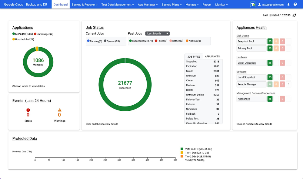
Backup is a fundamental aspect of application protection. As such, the need for a seamlessly integrated, centralized backup service is vital when seeking to ensure resilience and recoverability for data generated by Google Cloud services or on-premises infrastructure. Regardless of whether the need to restore data is triggered by a user error, malicious activity, or some other reason, the ability to execute reliable, fast recovery from backups is a critical aspect of a resilient infrastructure. A comprehensive backup capability should have the following characteristics: 1) centralized backup management across workloads, 2) efficient use of storage to minimize costs, and 3) minimal recovery times. To effectively address these requirements backup service providers must deliver efficiency at the workload level, while also supporting a diverse spectrum of customer environments, applications, and use cases. Consequently, the implementation of a truly effective, user-friendly backup experience is no small feat.And that’s why, today, we’re excited to announce the availability of Google Cloud Backup and DR, enabling centralized backup management directly from the Google Cloud console.Helping you maximize backup valueAt Google Cloud we have a unique opportunity to solve backup challenges in ways that fully maximize the value you achieve. By building a product with our customers firmly in mind, we’ve made sure that Google Cloud Backup and DR makes it easy to set up, manage, and restore backups.As an example, we placed a high priority on delivering an intuitive, centralized backup management experience. With Google Cloud Backup and DR, administrators can effectively manage backups spanning multiple workloads. Admins can generate application- and crash-consistent backups for VMs on Compute Engine, VMware Engine or on-premises VMware, databases (such as SAP, MySQL and SQL Server), and file systems. Having a holistic view of your backups across multiple workloads means you spend less time on management and can be sure you have consistency and completeness in your data protection coverage.Google Cloud Backup and DR dashboardEven better, Google Cloud Backup and DR stores backup data in its original, application-readable format. As a result, backup data for many workloads can be made available directly from long-term backup storage (e.g., leveraging cost-effective Cloud Storage), with no need for time-consuming data movement or translation. This accelerates recovery of critical files and supports rapid resumption of critical business operations.Making sure you minimize backup TCOSimilarly, we also took care to help you minimize total cost of ownership (TCO) of your backups. With this objective in mind, we designed Google Cloud Backup and DR to implement space-efficient “incremental forever” storage technology to ensure that you pay only for what you truly need. With “incremental forever” backup, after Google Cloud Backup and DR takes an initial backup, subsequent backups only store data associated with changes relative to the prior backup. This allows backups to be captured more quickly and reduces the network bandwidth required to transmit the associated data. It also minimizes the amount of storage consumed by the backups, which benefits you via reduced storage consumption costs.In addition, there is flexibility built in to allow you to strike your desired balance between storage cost and data retention time. For example, when choosing to store backups on Google Cloud Storage, you can select an appropriate Cloud Storage class in alignment with your needs.Start reaping the benefitsThe introduction of Google Cloud Backup and DR is a reflection of our broader commitment to make cloud infrastructure easier to manage, faster, and less expensive, while also helping you build a more resilient business. By centralizing backup administration and applying cutting-edge storage and data management technologies, we’ve eliminated much of the complexity, time, and cost traditionally associated with enterprise data protection.But don’t take our word for it. See for yourself in Google Cloud Console. Take advantage of $300 in free Google Cloud credits, give Google Cloud Backup and DR a try starting in late September 2022, and enjoy the benefits of cloud-integrated backup and recovery.Related ArticleNew storage innovations to drive your next-gen applicationsLearn about the latest products and features rolling out for customers using cloud-based block, file and object storage, as well as backu…Read Article
Quelle: Google Cloud Platform

Trust Update: September 2022

If you work in compliance, privacy, or risk, you know that regulatory developments have continued to accelerate this year. As part of our commitment to be the most trusted cloud, we continue to pursue global industry standards, frameworks, and codes of conduct that tackle our customers’ foundational need for a documented baseline of addressable requirements. We have seen key updates across all regions and have worked to help organizations address these new and evolving requirements. Let’s look at the significant updates from around the world, hot topics, and the requirements we’ve recently addressed.Global developments: Residency, portability, and moreGoogle Cloud meets or suprasses the standards for a number of frameworks including ISO/IEC 22301 for business continuity management and the Minimum Viable Secure Product(MVSP), developed with industry partners such as Salesforce, Okta, and Slack. Globally, we continue to address the areas of focus we know are most critical to organizations including operational resiliency, DPIA support, and international data transfers.Highlights from EMEA Consistent with what we have observed historically, EMEA remains a region full of ample developments that expand the regulatory landscape.Digital Operational Resilience Act (DORA) adopted for financial services organizations: One of our most recent critical announcements was our preparations for addressing DORA, which will harmonize how EU financial entities must report cybersecurity incidents, test their digital operational resilience, manage Information and Communications Technology (ICT) third-party risk, and allow financial regulators to directly oversee critical ICT providers. Second annual declaration of adherence to SWIPO: As presented in our SWIPO Transparency Statement, Google Cloud continues to demonstrate our commitment to enabling data portability and interoperability. Our customers always fully control their own data – including when they need to view, delete, download, and transfer their content.Supporting our EU education customers’ privacy assessments: The recent Datatilsynet (the Danish Data Protection Authority) ruling on proper due diligence of cloud services is a helpful reminder for customers to conduct thorough risk assessments of third parties. Our latest blog reaffirms Google Cloud’s commitment to helping Education customers and the rest of our current and potential customer base conduct due diligence, including supporting privacy assessments and independent third-party attestations. The introduction of new requirements in Asia PacificWe continue to monitor the rapidly evolving regulatory landscape in Asia Pacific that has been rich with new developments and the introduction of several laws so far this year. Addressed compliance for Australia’s DTA HCF: To help support Australian government customers with data residency and local customer support capabilities, Google Cloud is now ‘certified strategic’ under the Hosting Certification Framework (HCF) administered by Australia’s Digital Transformation Agency.Privacy requirements in Japan, New Zealand, and Taiwan: Meeting privacy obligations remain a top priority for many organizations. To help, we’ve built compliance support for Japan’s Act on the Protection of Personal Information (APPI) along with New Zealand’s Privacy Act and Taiwan’s Personal Data Protection Act (PDPA). Updated U.S. industry compliance In the United States, we continue to seek effective and efficient mechanisms to help our customers address their privacy and security needs. As with every region, customers can view our compliance offerings and mapping in our filterable Compliance Resource Center. Welcoming theTrans-Atlantic Data Privacy Framework: Following the framework implementation, Google Cloud reaffirmed our commitment to helping customers meet stringent data protection requirements. This includes making the protections offered by the E.U.-U.S. data transfer framework available to customers when available. New U.S. industry compliance mappings: From public sector (DISA), to health care (MARS-E), energy (NERC) and criminal justice (CJIS), we have reviewed U.S. industry requirements and released new materials outlining how we can help customers address compliance. A focus on Financial Services in Latin AmericaLatin America remains a focus this year, with Google’s June announcement committing $1.2 billion USD over 5 years to projects in the region. Later in July, Google Cloud built on these initiatives by announcing that a new Google Cloud region is coming to Mexico. For those in one of the most heavily regulated industries like financial services, we remain focused on demonstrating our commitment to regulations in that sector. Meeting outsourcing requirements in financial services: We have new and updated compliance mappings for banking requirements in Brazil, Peru, and Colombia. Each new mapping is designed to support risk and compliance leaders’ need for compliance and reporting documentation. Using our compliance developmentsWe know developments are impactful not only for organizations that seek to meet requirements, but also for those team members tasked with ensuring their service providers adapt their approaches in response to critical industry developments. Many Google Cloud customers are already using our trust and compliance resources to facilitate internal and external conversations with their key customers, business partners, and regulators. Visit our Compliance Resource Center or continue the conversation with our sales team by visiting our Sales Center today.Related ArticleGoogle Cloud’s preparations to address the Digital Operational Resilience ActAs the EU’s proposed DORA regulation reaches a major milestone, Google Cloud details our approach to its new rules and rule changes.Read Article
Quelle: Google Cloud Platform

Optimizing terabyte-scale PostgreSQL migrations to Cloud SQL with Searce

Google Cloud allows you to move your PostgreSQL databases to Cloud SQL with Database Migration Service (DMS). DMS gives you the ability to replicate data continuously to the destination database, while the source is live in production, enabling you to migrate with minimum downtime.However, terabyte-scale migrations can be complex. For instance, if your PostgreSQL database hasLarge Objects, then you will require some downtime to migrate them manually as that is a limitation of DMS. There are few more such limitations – check outknown limitations of DMS. If not handled carefully, these steps can extend the downtime during cutover, lead to performance impact on the source instance, or even delay the project delivery date. All this may mean significant business impact. Searce is a technology consulting company, specializing in modernizing application and database infrastructure by leveraging cloud, data and AI. We empower our clients to accelerate towards the future of their business. In our journey, we have helped dozens of clients migrate to Cloud SQL, and have found terabyte-scale migrations to be the toughest for the reasons mentioned earlier. This blog centers around our work in supporting an enterprise client whose objective was to migrate dozens of terabyte scale, mission-critical PostgreSQL databases to Cloud SQL with minimum downtime. Their largest database was 20TB in size and all the databases had tables with large objects and some tables did not have primary keys. Note that DMS had a limitation of not supporting migration of tables without a primary key during the time of this project. In June 2022, DMS released an enhancement to support the migration of tables without a primary key.  In this blog, we share with you our learnings about how we simplified and optimized this migration, so that you can incorporate our best practices into your own migrations. We explore mechanisms to reduce the downtime required for operations not handled by DMS by ~98% with the use of automation scripts. We also explore database flags in PostgreSQL to optimize DMS performance and minimize the overall migration time by ~15%. Optimize DMS performance with database flagsOnce the customer made the decision to migrate PostgreSQL databases to Google Cloud SQL, we considered two key factors that would decide business impact – migration effort and migration time. To minimize effort for the migration of PostgreSQL databases, we leveraged Google Cloud’s DMS (Database Migration Service) as it is very easy to use and  it does the heavy lifting by continuously replicating data from the source database to the destination Cloud SQL instance, while the source database is live in production.How about migration time? For a terabyte-scale database, depending on the database structure, migration time can be considerably longer. Historically, we observed that DMS took around 3 hours to migrate a 1 TB database. In other cases, where the customer database structure was more complex, migration took longer. Thankfully, DMS takes care of this replication while the source database is live in production, so no downtime is required during this time. Nevertheless, our client would have to bear the cost of both the source and destination databases which for large databases, might be substantial. Meanwhile, if the database size increased, then replication could take even longer, increasing the risk of missing the customer’s maintenance window for the downtime incurred during cutover operations. Since the customer’s maintenance window was monthly, we would have to wait for 30 more days for the next maintenance window, requiring the customer to bear the cost of both the databases for another 30 days. Furthermore, from a risk management standpoint, the longer the migration timeframe, the greater the risk that something could go wrong. Hence, we started exploring options to reduce the migration time. Even the slightest reduction in migration time could significantly reduce the cost and risk. We explored options around tuning PostgreSQL’s database flags on the source database. While DMS has its own set of prerequisite flags for the source instance and database, we also found that flags like shared_buffers, wal_buffers and maintenance_work_memhelped accelerate the replication process through DMS. These flags needed to be set to a specific value to get the maximum benefit out of each of them. Once set, their cumulative impact was a reduction in time for DMS to replicate a 1 TB database by 4 hours, that is, reduction of 3.5 days for a 20 TB database. Let’s dive into each of them.Shared BuffersPostgreSQL uses two buffers – its own internal buffer and the kernel buffered IO. In other words, that data is stored in memory twice. The internal buffer is called shared_buffers, and it determines the amount of memory used by the database for the operating system cache. By default this value is set conservatively low. However, increasing this value on the source database to fit our use case helped increase the performance of read heavy operations, which is exactly what DMS does once a job has been initialized.After multiple iterations, we found that if the value was set to 55% of the database instance RAM, it boosted the replication performance (a read heavy operation) by a considerable amount and in turn reduced the time required to replicate the data.WAL BuffersPostgreSQL relies on Write-Ahead Logging (WAL) to ensure data integrity. WAL records are written to buffers and then flushed to disk. The flag wal_buffers, determines the amount of shared memory used for WAL data that has not yet been written to disk – records that are yet to be flushed. We found that increasing the value for wal_buffers from the default value of 16MB to about 3% of the database instance’s RAM significantly improved the write performance by writing fewer but larger files to the disk at each transaction commit.Maintenance Work MemPostgreSQL maintenance operations, such as VACUUM, CREATE INDEX, and ALTER TABLE ADD FOREIGN KEY, consume their own specific memory. This memory is referred to as  maintenance_work_mem. Unlike other operations, PostgreSQL maintenance operations can only be performed sequentially by the database. Setting a value significantly higher than the default value of 64 MB meant that no maintenance operation would block the DMS job. We found that maintenance_work_mem worked best at the value of 1 GB.Resize source instance to avoid performance impactEach of these three flags tune how PostgreSQL utilizes memory resources. Hence, it was imperative that before setting these flags, we needed to upsize the source database instance to accommodate them. Without upsizing the database instances, we could have caused application performance degradation, as more than half of the total database memory would be allocated to the processes managed by these flags.We calculated the memory required by the flags mentioned above, and found that each flag needed to be set to a specific percentage of the source instance’s memory, irrespective of the existing values that might be set for the flags:shared_buffers: 55% of source instance’s memorywal_buffers: 3% of source instance’s memorymaintenance_work_mem: 1 GBWe added the individual memory requirements by the flags, and found that 58% of the RAM at least will be taken up by these memory flags. For example, if a source instance used 100GB of memory, 58GB would be taken up by shared_buffers and wal_buffers, and an additional 1GB by maintenance_work_mem. As the original value of these flags was very low (~200MB), we upsized the RAM of the source database instance by 60% in order to ensure that the migration did not impact source performance on the application live in production.Avoid connection error with WAL sender timeout flagWhile using Google Cloud’s DMS, if the connection is terminated between DMS and the Cloud SQL instance during the ‘Full Dump in Progress’ phase of the DMS job, the DMS job fails and needs to be reinitiated. Encountering timeouts, especially while migrating a terabyte-scale database, would mean multiple days’ worth of migration being lost and a delay in the cutover plan. For example, if the connection of the DMS job for a 20TB database migration is lost after 10 days, the DMS job will have to be restarted from the beginning, leading to 10 days’ worth of migration effort being lost.Adjusting the WAL sender timeout flag (wal_sender_timeout) helped us avoid terminating replication connections that were inactive for a long time during the full dump phase. The default value for this flag is 60 seconds. To avoid these connections from terminating, and to avoid such high impact failures, we set the value of this flag to 0 for the duration of database migration. This would avoid connections getting terminated and allowed for smoother replication through the DMS jobs.Generally, for all the database flags we talked about here, we advised our customer to restore the default flag values once the migration completed. Reduce downtime required for DMS limitations by automation While DMS does the majority of database migration through continuous replication when the source database instance is live in production, DMS has certain migration limitations that cannot be addressed when the database is live. For PostgreSQL, the known limitations of DMS include: Any new tables created on the source PostgreSQL database after the DMS job has been initialized are not replicated to the destination PostgreSQL database.Tables without primary keys on the source PostgreSQL database are not migrated. For those tables, DMS migrated only the schema. This is no longer a limitation after the June 2022 product update.The large object (LOB) data type is not supported by DMS.Only the schema for Materialized Views is migrated; the data is not migrated.All data migrated is created under the ownership of cloudsqlexternalsync.We had to address these aspects of the database migration manually. Since our client’s database had data with the large object data type, tables without primary keys, and frequently changing table structures that cannot be migrated by DMS, we had to manually export and import that data after DMS did most of the rest of the data migration. This part of database migration required downtime to avoid data loss. For a terabyte-scale database, this data can be in the hundreds of GBs, which means higher migration time and hence higher downtime. Furthermore, when you have dozens of databases to migrate, it can be stressful and error-prone for a human to perform these operations while on the clock during the cutover window! This is where automation helped save the day! Automating the migration operations during the downtime period not only reduced the manual effort and error risk, but also provided a scalable solution that could be leveraged for the migration of 100s of PostgreSQL database instances to Cloud SQL. Furthermore, by leveraging multiprocessing and multithreading, we were able to reduce the total migration downtime for 100s of GBs of data by 98%, thereby reducing the business impact for our client. How do we get there?We laid out all the steps that need to be executed during the downtime – that is, after the DMS job has completed its replication from source to destination and before cutting over the application to the migrated database. You can see a chart mapping out the sequence of operations that are performed during the downtime period in Fig 1.Fig 1: Downtime Migration – Sequential ApproachBy automating all the downtime operations in this sequential approach, we observed that it took 13 hours for the entire downtime flow to execute for a 1 TB database. This included the migration of 250 MB in new tables, 60 GB in tables without primary keys and 150 GB in large objects.  One key observation we made was that, out of all the steps, only three steps took most of the time: migrating new tables, migrating tables without primary keys, and migrating large objects. These took the longest time because they all required dump and restore operations for their respective tables. However, these three steps did not have a hard dependency on each other as they individually targeted different tables. So we tried to run them in parallel as you can see in Fig 2. But the steps following them – ‘Refresh Materialized View’ and ‘Recover Ownership’ – had to be performed sequentially as they targeted the entire database.However, running these three steps in parallel required upsizing the Cloud SQL instances, as we wanted to have sufficient resources available for each step. This led us to increase the Cloud SQL instances’ vCPU by 50% and memory by 40%, since the export and import operations depended heavily on vCPU consumption as opposed to memory consumption.Fig 2: Downtime Migrations – Hybrid ApproachMigrating the new tables (created after the DMS job was initiated) and tables without primary keys was straightforward as we were able to leverage the native utilities offered by PostgreSQL – pg_dump and pg_restore. Both utilities process tables in parallel by using multiple threads– the higher the table count, the higher the number of threads that could be executed in parallel, allowing faster migration. With this revised approach, for the same 1 TB database, it still took 12.5 hours for the entire downtime flow to execute. This improvement reduced the cutover downtime, but we still found that we needed a 12.5 hour window to complete all the steps. We then discovered that 99% of the time of downtime was taken up by just one step: exporting and importing 150 GB of large objects. It turned out that multiple threads could not be used to accelerate the dump and restore large objects in PostgreSQL. Hence, migrating the large objects single handedly extended the downtime for migration by hours. Fortunately, we were able to come up with a workaround for that. Optimize migration of Large Object from PostgreSQL databasePostgreSQL contains a large objects facility that provides stream-style access to data stored in a special large-object structure. When large objects are stored, they are broken down into multiple chunks and stored in different rows of the database, but are connected under a single Object Identifier (OID). This OID can thus be used to access any stored Large Object. Although users can add large objects to any table in the database, under the hood, PostgreSQL physically stores all large objects within a database in a single table called pg_largeobjects.While leveraging pg_dump and pg_restore for export and import of large objects, this single table – pg_largeobject, becomes a bottleneck as the PostgreSQL utilities cannot execute multiple threads for parallel processing, since it’s just one table. Typically, the order of operations for these utilities looks something like this:1. pg_dump reads the data to be exported from the source database 2. pg_dump writes that data into the memory of the client where pg_dump is being executed 3. pg_dump writes from memory to the disk of the the client (a second write operation)4. pg_restore reads the data from the client’s disk5. pg_restore writes the data to the destination databaseNormally, these utilities would need to be executed sequentially to avoid data loss or data corruption due to conflicting processes. This leads to further increase in migration time for large objects.Our workaround for this single-threaded process involved two elements. First, with our solution, we eliminated the second write operation – write from memory to disk (point #3). Instead, once the data was read and written into memory, our program would begin the import process and write data to the destination database. Second, since pg_dump and pg_restore could not use multiple threads to process the large objects in just the pg_largeobjects table, we took it upon ourselves to develop a solution that could use multiple threads. The thread count was based on the number of OIDs in the table – pg_largeobjects, and break that single table into smaller chunks for parallel execution. This approach brought down Large Object migration operation from hours to minutes, therefore bringing down the downtime needed for all operations to be completed that DMS cannot handle, for the same 1 TB database, from 13 hours to just 18 minutes. A reduction of ~98% in the required downtime.ConclusionAfter multiple optimizations and dry runs, we were able to develop a procedure for our client to migrate dozens of terabyte-scale PostgreSQL databases to Google Cloud SQL with a minimal business impact. We developed practices to optimize DMS-based migration by 15% using database flags and reduce downtime by 98% with the help of automation and innovation. These practices can be leveraged for any terabyte-scale migration of PostgreSQL databases to Google Cloud SQL to accelerate migration, minimize downtime and avoid performance impact on mission critical applications.Related ArticleRead Article
Quelle: Google Cloud Platform
Four non-traditional paths to a cloud career (and how to navigate them)

One thing I love about cloud is that it’s possible to succeed as a cloud engineer from all kinds of different starting points. It’s not necessarily easy; our industry remains biased toward hiring people who check a certain set of boxes such as having a university computer science degree. But cloud in particular is new enough, and has such tremendous demand for qualified talent, that determined engineers can and do wind up in amazing cloud careers despite coming from all sorts of non-traditional backgrounds.But still – it’s scary to look at all the experienced engineers ahead of you and wonder “How will I ever get from where I am to where they are?”A few months ago, I asked some experts at Google Cloud to help me answer common questions people ask as they consider making the career move to cloud. We recorded our answers in a video series called Cracking the Google Cloud Career that you can watch on the Google Cloud Tech YouTube channel. We tackled questions like…How do I go from a traditional IT background to a cloud job?You have a superpower if you want to move from an old-school IT job to the cloud: You already work in tech! That may give you access to colleagues and situations that can level up your cloud skills and network right in your current position. But even if that’s not happening, you don’t have to go back and start from square one. Your existing career will give you a solid foundation of professional experience that you can layer cloud skills on top of. Check out my video to see what skills I recommend polishing up before you make the jump to cloud interviews:How do I move from a help desk job to a cloud job?The help desk is the classic entry-level tech position, but moving up sometimes seems like an insurmountable challenge. Rishab Kumar graduated from a help desk role to a Technical Solutions Specialist position at Google Cloud. In his video, he shares his story and outlines some takeaways to help you plot your own path forward.Notably, Rishab calls out the importance of building a portfolio of cloud projects: cloud certifications helped him learn, but in the job interview he got more questions about the side projects he had implemented. Watch his full breakdown here:How do I switch from a non-technical career to the cloud?There’s no law that says you have to start your tech career in your early twenties and do nothing else for the rest of your career. In fact, many of the strongest technologists I know came from previous backgrounds as disparate as plumbing, professional poker, and pest control. That’s no accident: those fields hone operational and people skills that are just as valuable in cloud as anywhere else. But you’ll still need a growth mindset and lots of learning to land a cloud job without traditional credentials or previous experience in the space. Google Cloud’s Stephanie Wong came to tech from the pageant world and has some great advice about how to build a professional network that will help you make the switch to a cloud job. In particular, she recommends joining the no-cost Google Cloud Innovators program, which gives you inside access to the latest updates on Google Cloud services alongside a community of fellow technologists from around the globe.Stephanie also points out that you don’t have to be a software engineer to work in the cloud; there are many other roles like developer relations, sales engineers and solutions architects that stay technical and hands-on without building software every day.You can check out her full suggestions for transitioning to a tech career in this video:How do I get a job in the cloud without a computer-related college degree?No matter your age or technical skill level, it can be frustrating and intimidating to see role after role that requires a bachelor’s degree in a field such as IT or computer science. I’m going to let you in on a little secret: once you get that first job and add some experience to your skills, hardly anybody cares about your educational background anymore. But some recruiters and hiring managers still use degrees as a shortcut when evaluating people for entry-level jobs.Without a degree, you’ll have to get a bit creative in assembling credentials. First, consider getting certified. Cloud certifications like the Google Cloud Associate Cloud Engineer can help you bypass degree filters and get you an interview. Not to mention, they’re a great way to get familiar with the workings of your cloud. Google Cloud’s Priyanka Vergadia suggests working toward skill badges on Google Cloud Skills Boost; each skill badge represents a curated grouping of hands-on labs within a particular technology that can help you build momentum and confidence toward certification.Second, make sure you are bringing hands-on skills to the interview. College students do all sorts of projects to bolster their education. You can do this too – but at a fraction of the cost of a traditional degree. As Priyanka points out in this video, make sure you are up to speed on Linux, networking, and programming essentials before you apply:No matter your background, I’m confident you can have a fulfilling and rewarding career in cloud as long as you get serious about these two things:Own your credibility through certification and hands-on practice, andBuild strong connections with other members of the global cloud community.In the meantime, you can watch the full Cracking the Google Cloud Career playlist on the Google Cloud Tech YouTube channel. And feel free to start your networking journey by reaching out to me anytime on Twitter if you have cloud career questions – I’m happy to help however I can.Related ArticleShow off your cloud skills by completing the #GoogleClout weekly challengeComplete the weekly #GoogleClout challenge and show off your cloud skillsRead Article
Quelle: Google Cloud Platform
Pro tools for Pros: Industry leading observability capabilities for Dataflow

Dataflow is the industry-leading unified platform offering batch and stream processing. It is a fully managed service that comes with flexible development options (from Flex Templates & Notebooks to Apache Beam SDKs for Java, Python and Go) and a rich set of built-in management tools. It comes with seamless integrations with all Google Cloud products, such as Pub/Sub, BigQuery, VertexAI, GCS, Spanner, and BigTable, as well as third-party services and products, such as Kafka and AWS S3, to best meet your data movement use cases.While our customers value these capabilities, they continue to push us to innovate and provide more value as the best batch and streaming data processing service to meet their ever-changing business needs. Observability is a key area where the Dataflow team continues to invest more based on customer feedback. Adequate visibility into the state and performance of the Dataflow jobs is essential for business critical production pipelines. In this post, we will review Dataflow’s  key observability capabilities:Job visualizers – job graphs and execution detailsNew metrics & logsNew troubleshooting tools – error reporting, profiling, insightsNew Datadog dashboards & monitorsDataflow observability at a glanceThere is no need to configure or manually set up anything; Dataflow offers observability out of the box within the Google Cloud Console, from the time you deploy your job. Observability capabilities are seamlessly integrated with Google Cloud Monitoring and Logging along with other GCP products. This integration gives you a one-stop shop for observability across multiple GCP products, which you can use to meet your technical challenges and business goals.Understanding your job’s execution: job visualizersQuestions: What does my pipeline look like? What’s happening in each step? Where’s the time spent?Solution: Dataflow’s Job graph and Execution details tabs answer these questions to help you understand the performance of various stages and steps within the jobJob graph illustrates the steps involved in the execution of your job, in the default Graph view. The graph gives you a view of how Dataflow has optimized your pipeline’s code for execution, after fusing  (optimizing) steps to stages. TheTable view informs you more about each step and the associated fused stages and time spent in each step and their statuses as the pipeline continues execution. Each step in the graph displays more information, such as the input and output collections and output data freshness; these help you analyze the amount of work done at this step (elements processed) and the throughput for it.Fig 1. Job graph tab showing the DAG for a job and the key metrics for each stage on the right.Execution Details has all the information to help you understand and debug the progress of each stage within your job. In the case of streaming jobs, you can view the data freshness of each stage. The Data freshness by stages chart includes anomaly detection: it highlights “potential slowness” and “potential stuckness” to help you narrow down your investigation to a particular stage. Learn more about using the Execution details tab for batch and streaming here.Fig 2. The execution details tab showing data freshness by stage over time, providing anomaly warnings in data freshness.Monitor your job with metrics and logsQuestions:  What’s the state and performance of my jobs? Are they healthy? Are there any errors? Solution:  Dataflow offers several metrics to help you monitor your jobs. A full list of Dataflow job metrics can be found in our metrics reference documentation. In addition to the Dataflow service metrics, you can view worker metrics, such as CPU utilization and memory usage. Lastly, you can generate Apache Beam custom metrics from your code.Job metrics is the one-stop shop to access the most important metrics for reviewing the performance of a job or troubleshooting a job. Alternatively, you can access this data from the Metrics Explorer to build your own Cloud Monitoring dashboards and alerts. Job and worker Logs are one of the first things that you can look at when you deploy a pipeline. You can access both these log types in the Logs panel on the Job details page. Job logs include information about startup tasks, fusion operations, autoscaling events, worker allocation, and more. Worker logs include information about work processed by each worker within each step in your pipeline.You can configure and modify the logging level and route the logs using the guidance provided in our pipeline log documentation. Logs are seamlessly integrated into Cloud Logging. You can write Cloud Logging queries, create log-based metrics, and create alerts on these metrics. New: Metrics for streaming JobsQuestions: Is my pipeline slowing down or getting stuck? I want to understand how my code is impacting the job’s performance. I want to see how my sources and sinks are performing with respect to my jobSolution: We have introduced several new metrics for Streaming Engine jobs that help answer these questions. Notable metrics are listed below. All of these are now instantly accessible from the Job metrics tab.The engineering teams at the Renault Group have been using Dataflow for their streaming pipelines as a core part of their digital transformation journey.”Deeper observability of our data pipelines is critical to track our application SLOs,”said Elvio Borrelli, Tech Lead – Big Data at the Renault Digital Transformation & Data team. “The new metrics, such as backlog seconds and data freshness by stage, now provide much better visibility about our end-to-end pipeline latencies and areas of bottlenecks. We can now focus more on tuning our pipeline code and data sources for the necessary throughput and lower latency”.To learn more about using these metrics in the Cloud console, please see the Dataflow monitoring interface documentation.Fig 3. The Job metrics tab showing the autoscaling chart and the various metrics categories for streaming jobs.To learn how to use these metrics to troubleshoot common symptoms within your jobs, watch this webinar on Dataflow Observability: Dataflow Observability, Monitoring, and Troubleshooting Debug job health using Cloud Error ReportingProblem: There are a couple of errors in my Dataflow job. Is it my code, data, or something else? How frequently are these happening?Solution: Dataflow offers native integration with Google Cloud Error Reporting to help you identify and manage errors that impact your job’s performance.In the Logs panel on the Job details page, the Diagnostics tab tracks the most frequently occurring errors. This is integrated with Google Cloud Error Reporting, enabling you to manage errors by creating bugs or work items or by setting up notifications. For certain types of Dataflow errors, Error Reporting provides a link to troubleshooting guides and solutions.Fig 4. The diagnostics tab in the Log panel displaying top errors and their frequency.New: Troubleshoot performance bottlenecks using Cloud ProfilerProblem: What part of my code is taking more time to process the data? What operations are consuming more CPU cycles or memory?Solution: Dataflow offers native integration with Google Cloud Profiler, which lets you profile your jobs to understand the performance bottlenecks using CPU, memory, and I/O operation profiling support.Is my pipeline’s latency high? Is it CPU intensive or is it spent time waiting for I/O operations? Or is it memory intensive? If so, which operations are driving this up? The flame graph helps you find answers to these questions. You can enable profiling for your Dataflow jobs by specifying a flag during job creation or while updating your job. To learn more see the Monitor pipeline performance documentation.Fig 5. The CPU time profiler for showing the flame graph for the Dataflow job.New: Optimize your jobs using Dataflow insightsProblem: What can Dataflow tell me about improving my job performance or reducing its costs?Solution: You can review Dataflow Insights to improve performance or to reduce costs. Insights are enabled by default on your batch and streaming jobs; they are generated by auto-analyzing your jobs’ executions.Dataflow insights is powered by the Google Active Assist’s Recommender service. It is automatically enabled for all jobs and is available free of charge. Insights include recommendations such as enabling autoscaling, increasing maximum workers, and increasing parallelism. Learn more about Dataflow insights in the Dataflow Insights documentation.Fig 6. Dataflow Insights show up in  the Jobs overview page next to the active jobs.New: Datadog Dashboards & Recommended MonitorsProblem: I would like to monitor Dataflow in my existing monitoring tools, such as Datadog.Solution: Dataflow’s metrics and logs are accessible in observability tools of your choice, via Google Cloud Monitoring and Logging APIs. Customers using Datadog can now leverage the out of the box Dataflow dashboards and recommended monitors to monitor their Dataflow jobs alongside other applications within the Datadog console. Learn more about Dataflow Dashboards and Recommended Monitors in their blog post on how to monitor your Dataflow pipelines with Datadog.Fig 7. Datadog dashboard monitoring Dataflow jobs across projectsZoomInfo, a global leader in modern go-to-market software, data, and intelligence, is partnering with Google Cloud to enable customers to easily integrate their business-to-business data into Google BigQuery. Dataflow is a critical piece of this data movement journey.“We manage several hundreds of concurrent Dataflow jobs,” said Hasmik Sarkezians, ZoomInfo Engineering Fellow. “Datadog’s dashboards and monitors allow us to easily monitor all the jobs at scale in one place. And when we need to dig deeper into a particular job, we leverage the detailed troubleshooting tools in Dataflow such as Execution details, worker logs and job metrics to investigate and resolve the issues.”What’s NextDataflow is leading the batch and streaming data processing industry with the best in class observability experiences. But we are just getting started. Over the next several months, we plan to introduce more capabilities such as:Memory observability to detect and prevent potential out of memory errors.Metrics for sources & sinks, end-to-end latency, bytes being processed by a PTransform, and more.More insights – quota, memory usage, worker configurations & sizes.Pipeline validation before job submission.Debugging user-code and data issues using data sampling.Autoscaling observability improvements.Project-level monitoring, sample dashboards, and recommended alerts.Got feedback or ideas? Shoot them over, or take this short survey.Getting StartedTo get started with Dataflow see the  Cloud Dataflow quickstarts.To learn more about Dataflow observability, review these articles:Using the Dataflow monitoring interfaceBuilding production-ready data pipelines using Dataflow: Monitoring data pipelinesBeam College: Dataflow MonitoringBeam College: Dataflow Logging Beam College: Troubleshooting and debugging Apache Beam and GCP Dataflow
Quelle: Google Cloud Platform

Spanner on a modern columnar storage engine

Google was born in the cloud. At Google, we have been running massive infrastructure that powers critical internal and external facing services for more than two decades. Our investment in this infrastructure is constant, ranging from user visible features to invisible internals that makes the infrastructure more efficient, reliable and secure. Constant updates and improvements are made into the infrastructure. With billions of users served around the globe, availability and reliability is at the core of how we operate and update our infrastructure.Spanner is Google’s massively scalable, replicated and strongly consistent database management service. With hundreds of thousands of databases running in our production instance, Spanner serves over 2 billion requests at peak and has over 6 exabytes of data under management that is the “source of the truth” for many mission critical services, including AdWords, Search, and Cloud Spanner customers. The customer workloads are diverse, and would stretch a system in various ways. Although there have been constant binary releases to Spanner, fundamental changes such as swapping out the underlying storage engine is a challenging undertaking.  In this post, we talk about our journey migrating Spanner to a new columnar storage engine. We discuss the challenges a massive scale migration faced and how we accomplished this effort in ~2-3 years with all the critical services running on top uninterrupted.The Storage EngineThe storage engine is where a database turns their data into actual bytes and stores them in underlying file systems. In a Spanner deployment, a database is hosted in one or more instance configurations, which are physical collections of resources. The instance configurations and databases comprise one or more zones or replicas that are served by a number of spanner servers. The storage engine in the server encodes the data and stores them in the underlying large scale distributed file system – Colossus.Spanner originally used a Bigtable-like storage engine based on SSTable (Sorted String Table) format stacks. This format has proven to be incredibly robust through years of large scale deployment such as in Bigtable and Spanner itself. The SSTable format is optimized for schemaless NoSQL data consisting of primarily large strings. While it is a perfect match for Bigtable, it is not the best fit for Spanner. In particular, traversing individual columns is inefficient.Ressi is the new low-level, column-oriented storage format for Spanner. It is designed from the ground up for handling SQL queries over large-scale, distributed databases with both OLTP and OLAP workloads, including maintaining and improving performance of read and write queries with key-value data in the database. Ressi includes optimizations ranging from block-level data layout, file-level organization of active and inactive data, and existence filters for storage I/O savings etc. The data organization improves storage usage and helps in large scan queries. Deployment of Ressi with very large scale services such as GMail on Spanner have shown performance improvements over multiple dimensions, such as CPU and storage I/O.The Challenges of Storage Engine MigrationImprovements and updates to Spanner are constant and we are adept at safely operating and evolving our system in a dynamic environment. However, a storage engine migration changes the foundation of a database system and presents distinct challenges, especially at a massive deployment scale.In general, in a production OLTP database system, storage engine migration needs to be done without interruption to the hosted databases, without degradation to latency and throughput, and without compromising data integrity. There had been past attempts and success stories of live database storage engine migration. However, successful attempts at the scale of Spanner with multiple exabytes of data are rare. The mission critical nature of the services and the massive scale place a very high requirement on how the migration should be handled.Reliability, Availability & Data IntegrityThe topmost requirement of the migration is maintaining service reliability, availability and data integrity throughout the migration. The challenges were paramount and unique with the massive deployment scale of Spanner:Spanner database workloads are diverse and interact with the underlying Spanner system in different ways. Successful migration of one database does not guarantee successful migration of another.Massive data migration inherently creates unusual churns in the underlying system. This may trigger latent and unanticipated behavior, causing production outages.We operate in a dynamic environment with constant new ambient changes from the customers and Spanner new feature development. Migration faced non-monotonically decreasing risk.Performance & CostAnother challenge of migrating to a new storage engine is to achieve good performance and reduce cost. Performance regression can arise during the migration from underlying churns, and/or after the migration due to certain aspects of the workloads interacting with the new storage engine. This can cause issues such as increased latency and rejected requests.Performance regression may also manifest as increased storage usage in some databases due to variances in database compressibility. This increases internal resource consumption and cost. What’s more, if additional storage is not available, it may lead to production outages.Although the new columnar storage engine improves both performance and data compression in general, due to Spanner’s massive deployment, we must watch out for the outliers.Complexity and SupportabilityExistence of dual formats not only requires more engineering effort to support, but also increases system complexity and performance variances in different zones. An obvious approach to mitigate the risk here is to achieve high migration velocity and in particular, shorten the co-existence of dual formats in the same databases.However, databases on Spanner have different sizes, spanning several orders of magnitude. As a result, the time required to migrate each database can vary by a large degree. Scheduling databases for migration can not be done one-size-fit-all. The migration effort must take into account the transitioning period where dual formats exist while trying to achieve highest velocity safely and reliably.A Systematic Principled Approach toward Migration ReliabilityWe introduced a systematic approach based on a set of reliability principles we defined. Using the reliability principles, our automation framework automatically evaluated migration candidates (i.e., instance configurations and/or databases), selecting conforming candidates for migration and flagging violations. The flagged migration candidates were specially examined and violations resolved before the candidates became eligible for migration. This effectively reduced toil and increased velocity without sacrificing production safety.The Reliability Principles & Automation ArchitectureThe reliability principles were the cornerstones of how we conducted the migration. They covered multiple aspects: from evaluating the healthiness and suitability of migration candidates, managing customer exposure to production changes, handling performance regression and data integrity, to mitigating risks in a dynamic environment with constant changes, such as new releases and feature launches within and outside of Spanner.Based on the reliability principles, we built an automation framework. Various stats and metrics were collected. Together they formed a modeled view of the state of the Spanner universe. This view was continuously updated to accurately reflect the current state of the universe.In this architectural design, the reliability principles became filters, where a migration candidate could only pass through and be selected by the migration scheduler if it satisfied the requirements. Migration scheduling was done in weekly waves to enable gradual rollout.As previously mentioned, migration candidates not satisfying the reliability principles were not ignored – they were flagged for attention and were resolved in one of two ways: override and migrate with caution, or resolve the underlying blocking issue then migrate.Migration Scheduling & Weekly RolloutMigration scheduling was the core component in managing migration risk, preventing performance regressions and ensuring data integrity.Due to the diverse customer workload and wide spectrum of deployment sizes, we adopted fine-grained migration scheduling. The scheduling algorithm observed the customer deployment as failure domains and properly staged and spaced the migration of customer instance configurations. Together with the rollout automation, they enabled an efficient migration journey while keeping risk under control.Under this framework, the migration proceeded progressively in the following dimensions:among multiple instance configurations of the same customer deployment;among the multiple zones of the same instance configuration; andamong the migration candidates in the weekly rollout wave.Customer Deployment-aware SchedulingProgressive rollout within a customer’s deployment required us to recognize the customer deployment as failure domains. We used an heuristic that indicates deployment ownership and usage. In Spanner’s case, this is also a close approximation of workload categorization as the multiple instances are typically regional instances of the same service. The categorization produced equivalent classes of deployment instances where each class is a collection of instance configurations from the same customer and with the same workload, as shown in a simplified graph:The weekly wave scheduler selected migration candidates (i.e., replicas/zones in instance configuration) from each equivalent class. Candidates from multiple equivalent classes can be chosen independently as their workloads were isolated. Blocking issues in one equivalent class would not prevent progress in other classes.Progressive Rollout of Weekly WavesTo mitigate new issues from new releases and changes from both customers and Spanner, the weekly waves were also rolled out in a progressive manner, allowing issues to surface without causing widespread impact while accelerating to increase migration velocity.Managing Reliability, Availability & PerformanceUnder the mechanisms described above, customer deployments were carefully moved through a series of state changes, preventing performance degradation and loss of availability and data integrity.At the start, an instance configuration of a customer was chosen and an initial zone/replica ( henceforth referred to as “first zone”) was migrated. This avoided potential global production impact to the customer while revealing issues should the workload interact poorly with the new storage engine. Following the first zone migration, data integrity was checked by comparing the migrated zone with other zones using Spanner’s built-in integrity check. If this check failed or performance regression occurred following the migration, the instance was restored to the previous state.We pre-estimated the post migration storage size and the reliability principle blocks instances with excessive storage increase from migrating. As a result, we did not have many unexpected storage compression regression following a migration. Regardless, the resource usage and system health was closely monitored by our monitoring infrastructure. If unexpected regression occurred, the instance was restored back to the desired state by migrating the zone back to SSTable format.Only when everything was OK would the migration of the customer deployment proceed forward, progressively by migrating more instances and/or zones, and accelerating as risk was further reduced.Project Management & Driving MetricsA massive migration effort requires effective project management and the identification of key metrics to drive progress. We drove a few key metrics, including (but not limited to):The coverage metric. This metric tracked the number and percentage of Spanner instances running the new storage engine. This was the highest priority metric. As the name indicated, this metric covered the interaction of different workloads with the new storage engine, allowing early discovery of underlying issues.The majority metric. This metric tracked the number and percentage of Spanner instances with the majority of the zones running the new storage engine. This allows catching anomalies at tipping points in a quorum based system like Spanner.The completion metric. This metric tracked the number and percentage of Spanner instances that were completely running the new storage engine. Achieving 100% on this metric was our ultimate goal.The metrics were maintained as time series, allowing examination of the trend and shifting gears as we approached the later stages of the effort.SummaryPerforming massive scale migration is an effort that encompasses strategic design, building automation, designing processes, and shifting execution gears as effort progresses. With a systematic and principled approach, we achieved a massive scale migration involving over 6 exabytes of data under management and 2 billion QPS at peak in Spanner within a short amount of time with service availability, reliability and integrity uncompromised.Many of Google’s critical services depend on Spanner and have already seen significant improvements with this migration. Furthermore, the new storage engine provides a platform for many future innovations. The best is yet to come.
Quelle: Google Cloud Platform

Cloud Wisdom Weekly: 5 ways to reduce costs with containers

“Cloud Wisdom Weekly: for tech companies and startups” is a new blog series we’re running this fall to answer common questions our tech and startup customers ask us about how to build apps faster, smarter, and cheaper. In this installment, Google Cloud Product Manager Rachel Tsao explores how to save on compute costs with modern container platforms. Many tech companies and startups are built to operate under a certain degree of pressure and to efficiently manage costs and resources. These pressures have only increased with inflation, geopolitical shifts, and supply chain concerns, however, creating urgency for companies to find ways to preserve capital while increasing flexibility. The right approach to containers can be crucial to navigating these challenges. In the last few years, development teams have shifted from virtual machines (VMs) to containers, drawn to the latter because they are faster, more lightweight, and easier to manage and automate. Containers also consume fewer resources than VMs, by leveraging shared operating systems. Perhaps most importantly, containers enable portability, letting developers put an application and all its dependencies into a single package that can run almost anywhere. Containers are central to an organization’s agility, and in our conversations with customers about why they choose Google Cloud, we hear frequently that services like Google Kubernetes Engine (GKE) and Cloud Run help tech companies and startups to not only go to market quickly, but also save money. In this article, we’ll explore five ways to help your business quickly and easily reduce compute costs with containers. 5 ways to control compute costs with containers Whether your company is  an established player that is modernizing its business or a startup building its first product, managed containerized products can help you reduce costs, optimize development, and innovate. The following tips will help you to evaluate core features you should expect of container services and include specific advice for GKE and Cloud Run.1. Identify opportunities to reduce cluster administration Most companies want to dedicate resources to innovation, not infrastructure curation. If your team has existing Kubernetes knowledge or runs workloads that need to leverage machine types or graphics processing units (GPUs), you may be able to simplify provisioning with GKE Autopilot. GKE Autopilot provisions and manages the cluster’s underlying infrastructure, all while you pay for only the workload, not 24/7 access to the underlying node-pool compute VMs. In this way, it can reduce cluster administration while saving you money and giving you hardened security best practices by default.2. Consider serverless to maximize developer productivity Serverless platforms continue the theme of empowering your technical talent to focus on the most impactful work. Such platforms can promote productivity by abstracting away aspects of infrastructure creation, letting developers work on projects that drive the business while the platform provider oversees hardware and scalability, aspects of security, and more.  For a broad range of workloads that don’t need machine types or GPUs, going serverless with Cloud Run is a great option for building applications, APIs, internal services, and even real-time data pipelines. Analyst research supports that Cloud Run customers achieve faster deployments with less time spent monitoring services, resulting in reinvested productivity that lets these customers do more with fewer resources.  Designed with high scalability in mind, and an emphasis on the portability of containers, Cloud Run also supports a wide range of stateless workloads, including jobs that run to completion. Moreover, it lets you maximize the skills of your existing team, as it does not require cluster management, a Kubernetes skillset or prior infrastructure experience. Additionally, Cloud Run leverages the Knative spec and a container image as a deployment artifact, enabling an easy migration to GKE if your workload needs change.With Cloud Run, gone are the days of infrastructure overprovisioning! The platform scales down to zero automatically, meaning your services always have the capacity to meet demand, but do not incur costs if there is no traffic. 3. Save with committed use discountsCommitted use discounts provide discounted pricing in exchange for committing to a minimal level of usage in a region for a specified term. If you are able to reliably predict your resource needs, for instance, you can get a 17% discount for Cloud Run (for either one year or three years), and either a 20% discount (for one year) or a 45% discount (for three years) on GKE Autopilot.4. Leverage cost management features Minimum and maximum instances are useful for ensuring your services are ready to receive requests but do not cause cost overages. For Google Cloud customers, best practices for cost management include building your container with Cloud Build, which offers pay-for-use pricing and can be more cost efficient than steady-state build farms.Relatedly, if you choose to leverage serverless containers with Cloud Run, you can set minimum instances to avoid the lag (i.e., the cold start) when a new container instance is starting up from zero. Minimum instances are billed at one-tenth of the general Cloud Run cost. Likewise, if you are testing and want to avoid costs spiraling, you can set a maximum number of instances to ensure your containers do not scale beyond a certain threshold. These settings can be turned off anytime, resulting in no costs when your service is not processing traffic. To have better oversight of costs, you can also view built-in billing reports and set budget alerts on Cloud Billing. 5. Match workload needs to pricing modelsGKE Autopilot is great for running highly reliable workloads thanks to its Pod-level SLA. But if you have workloads that do not need a high level of reliability (e.g., fault tolerant batch workloads, dev/test clusters), you can leverage spot pricing to receive a discount of 60% to 91% compared to regularly-priced pods. Spot Pods run on spare Google Cloud compute capacity as long as resources are available. GKE will evict your Spot Pod with a grace period of 25 seconds during times of high resource demand, but you can automatically redeploy as soon as there is available capability. This can result in significant savings for workloads that are a fit. Innovation requires balance Put into practice, these tips can help you and your business to get the most out of containers while controlling management and resource costs. That said, it is worth noting that while managing cloud costs is important, the relationship between “cloud” and “cost” is often complex. If you are adopting cloud computing with only the primary goal of saving money, you may soon run into other challenges. Cloud services can save your business money in many ways, but they can also help you get the most value for your money. This balance between cost efficiency and absolute cost is important to keep in mind so that even in challenging economic landscapes, your tech company or startup can continue growing and innovating. Beyond cost savings, many tech and startup companies are seeking improved business agility, which is the ability to deploy new products and features frequently and with high quality. With deployment best practices built into GKE Autopilot and Cloud Run, you can transform the way your team operates while maximizing productivity with every new deployment. You can learn if your existing workloads are appropriate for containers with this fit assessment and these guides for migrating to containers. For new workloads, you can leverage these guides for GKE Autopilot and Cloud Run. And for more tips on cost optimization, check out our Architecture Framework for compute, containers, and serverless.If you want to learn more about how Google Cloud can help your startup, visit our page here to get more information about our program and apply for our Google for Startups Cloud Program, and sign up for our communications to get a look at our community activities, digital events, special offers, and more.Related ArticleThink serverless: tips for early-stage startupsGoogle Cloud tips for early-stage startups, from leveraging serverless to maximizing cloud credits to comparing managed services.Read Article
Quelle: Google Cloud Platform

Integrating ML models into production pipelines with Dataflow

Google Cloud’s Dataflow recently announced the General Availability support for Apache Beam’s generic machine learning prediction and inference transform, RunInference. In this blog, we will take a deeper dive on the transform, including:Showing the RunInference transform used with a simple model as an example, in both batch and streaming mode.Using the transform with multiple models in an ensemble.Providing an end-to-end pipeline example that makes use of an open source model from Torchvision. In the past, Apache Beam developers who wanted to make use of a machine learning model locally, in a production pipeline, had to hand-code the call to the model within a user defined function (DoFn), taking on the technical debt for layers of boilerplate code. Let’s have a look at what would have been needed:Load the model from a common location using the framework’s load method.Ensure that the model is shared amongst the DoFns, either by hand or via the shared class utility in Beam.Batch the data before the model is invoked to improve the model efficiency. The developer would set this up, either by hand or via one of the groups into batches utilities.Provide a set of metrics from the transform.Provide production grade logging and exception handling with clean messages to help that SRE out at 2 in the morning! Pass specific parameters to the models, or start to build a generic transform that allows the configuration to determine information within the model. And of course these days, companies need to deploy many models, so the data engineer begins to do what all good data engineers do and builds out an abstraction for the models. Basically, each company is building out their own RunInference transform!  Recognizing that all of this activity is mostly boilerplate regardless of the model, the RunInference API was created. The inspiration for this API comes from the tfx_bsl.RunInference transform that the good folks over at TensorFlow Extended built to help with exactly the issues described above. tfx_bsl.RunInference was built around TensorFlow models. The new Apache Beam RunInference transform is designed to be framework agnostic and easily composable in the Beam pipeline. The signature for RunInference takes the form of RunInference(model_handler), where the framework-specific configuration and implementation is dealt with in the model_handler configuration object. This creates a clean developer experience and allows for new frameworks to be easily supported within the production machine learning pipeline, without disrupting the developer workflow.. For example, NVIDIA is contributing to the Apache Beam project to integrateNVIDIA TensorRTTM, an SDK that can optimize trained models for deployment with the highest throughput and lowest latency on NVIDIA GPUs within Google Dataflow (PullRequest).  Beam Inference also allows developers to make full use of the versatility of Apache Beam’s pipeline model, making it easier to build complex multi-model pipelines with minimum effort. Multi-model pipelines are useful for activities like A/B testing and building out ensembles. For example, doing natural language processing (NLP) analysis of text and then using the results within a domain specific model to drive a customer recommendation. In the next section, we start to explore the API using code from the public codelab with the notebook also available at github.com/apache/beam/examples/notebooks/beam-ml.Using the Beam Inference APIBefore we get into the API, for those who are unfamiliar with Apache Beam, let’s put together a small pipeline that reads data from some CSV files to get us warmed up on the syntax.code_block[StructValue([(u’code’, u”import apache_beam as beamrnrnwith beam.Pipeline() as p:rn data = p | beam.io.ReadFromText(‘./file.csv’) rn data | beam.Map(print)”), (u’language’, u”), (u’caption’, <wagtail.wagtailcore.rich_text.RichText object at 0x3eaaa26ab6d0>)])]In that pipeline, we used the ReadFromText source to consume the data from the CSV file into a Parallel Collection, referred to as a PCollection in Apache Beam. In Apache Beam syntax, the pipe ‘|’ operator essentially means “apply”, so the first line applies the ReadFromText transform. In the next line, we use a beam.Map() to do element-wise processing of the data; in this case, the data is just being sent to the print function.Next, we make use of a very simple model to show how we can configure RunInference with different frameworks. The model is a single-layer linear regression that has been trained on y = 5x data (yup, it’s learned its fives times table). To build this model, follow the steps in the codelab. The RunInference transform has the following signature: RunInference(ModelHandler). The ModelHandler is a configuration that informs RunInference about the model details and that provides type information for the output. In the codelab, the PyTorch saved model file is named ‘five_times_table_torch.pt’ and is output as a result of the call to torch.save() on the model’s state_dict. Let’s create a ModelHandler that we can pass to RunInference for this model:code_block[StructValue([(u’code’, u”my_handler = PytorchModelHandlerTensor(rn state_dict_path=./five_times_table_torch.pt,rn model_class=LinearRegression,rn model_params={‘input_dim': 1,rn ‘output_dim': 1}”), (u’language’, u”), (u’caption’, <wagtail.wagtailcore.rich_text.RichText object at 0x3eaa926196d0>)])]The model_class is the class of the PyTorch model that defines the model architecture as a subclass of torch.nn.Module. The model_params are the ones that are defined by the constructor of the model_class. In this example, they are used in the notebook LinearRegression class definition:code_block[StructValue([(u’code’, u’class LinearRegression(torch.nn.Module):rn def __init__(self, input_dim=1, output_dim=1):rn super().__init__()rn self.linear = torch.nn.Linear(input_dim, output_dim) rn def forward(self, x):rn out = self.linear(x)rn return out’), (u’language’, u”), (u’caption’, <wagtail.wagtailcore.rich_text.RichText object at 0x3eaaa25e92d0>)])]The ModelHandler that is used also provides the transform information about the input type to the model, with PytorchModelHandlerTensor expecting torch.Tensor elements.To make use of this configuration, we update our pipeline with the configuration. We will also do the pre-processing needed to get the data into the right shape and type for the model that has been created. The model expects a torch.Tensor of shape [-1,1] and the data in our CSV file is in the format 20,30,40.code_block[StructValue([(u’code’, u”with beam.Pipeline() as p:rn raw_data = p | beam.io.ReadFromText(‘./file.csv’)rn shaped_data = raw_data | beam.FlatMap(lambda x : rn [numpy.float32(y).reshape(-1,1) rn for y in x.split(‘,’)]))rn results = shaped_data | beam.Map(torch.Tensor) | RunInference(my_handler)rn results | beam.Map(print)”), (u’language’, u”), (u’caption’, <wagtail.wagtailcore.rich_text.RichText object at 0x3eaa91962f50>)])]This pipeline will read the CSV file, get the data into shape for the model, and run the inference for us. The result of the print statement can be seen here:PredictionResult(example=tensor([20.]), inference=tensor([100.0047], grad_fn=<UnbindBackward0>))The PredictionResult object contains both the example as well as the result, in this case 100.0047 given an input of 20. Next, we look at how composing multiple RunInference transforms within a single pipeline gives us the ability to build out complex ensembles with a few lines of code. After that, we will look at a real model example with TorchVision.Multi model pipelinesIn the previous example, we had one model, a source, and an output. That pattern will be used by many pipelines. However, business needs also require ensembles of models where models are used for pre-processing of the data and for the domain specific tasks. For example, conversion of speech to text before being passed to an NLP model. Though the diagram above is a complex flow, there are actually three primary patterns. 1- Data is flowing down the graph.2- Data can branch after a stage, for example after ‘Language Understanding’.3- Data can flow from one model into another.Item 1 means that this is a good fit for building into a single Beam pipeline because it’s acyclic. For items 2 and 3, the Beam SDK can express the code very simply. Let’s take a look at these.Branching Pattern:In this pattern, data is branched to two models. To send all the data to both models, the code is in the form:code_block[StructValue([(u’code’, u’model_a_predictions = shaped_data | RunInference(configuration_model_a)rn model_b_predictions = shaped_data | RunInference(configuration_model_b)’), (u’language’, u”), (u’caption’, <wagtail.wagtailcore.rich_text.RichText object at 0x3eaaa2307890>)])]Models in Sequence:In this pattern, the output of the first model is sent to the next model. Some form of post processing normally occurs between these stages. To get the data in the right shape for the next step, the code is in the form:code_block[StructValue([(u’code’, u’model_a_predictions = shaped_data | RunInference(configuration_model_a)rnmodel_b_predictions = (model_a_predictions | beam.Map(postprocess) rn | RunInference(configuration_model_b))’), (u’language’, u”), (u’caption’, <wagtail.wagtailcore.rich_text.RichText object at 0x3eaaa031ff50>)])]With those two simple patterns (branching and model in sequence) as building blocks, we see that it’s possible to build complex ensembles of models. You can also make use of other Apache Beam tools to enrich the data at various stages in these pipelines. For example, in a sequential model, you may want to join the output of model a with data from a database before passing it to model b, bread and butter work for Beam. Using an open source modelIn the first example, we used a toy model that was available in the codelab. In this section, we walk through how you could use an open source model and output the model data to a Data Warehouse (Google Cloud BigQuery) to show a more complete end-to-end pipeline.Note that the code in this section is self-contained and not part of the codelab used in the previous section. The PyTorch model we will use to demonstrate this is maskrcnn_resnet50_fpn, which comes with Torchvision v 0.12.0. This model attempts to solve the image segmentation task: given an image, it detects and delineates each distinct object appearing in that image with a bounding box.In general, libraries like Torchvision pretrained models download the pretrained model directly into memory. To run the model with RunInference, we need a different setup, because RunInference will load the model once per Python process to be shared amongst many threads. So if we want to use a pre-trained model from these types of libraries, we have a little bit of setup to do. For this PyTorch model we need to:1- Download the state dictionary and make it available independently of the library to Beam.2- Determine the model class file and provide it to our ModelHandler, ensuring that we disable the class’s ‘autoload’ features.When looking at the signature for this model with version 0.12.0, note that there are two parameters that initiate an auto-download: pretrained and pretrained_backbone. Ensure these are both set to False to make sure that the model class does not load the model files:model_params = {‘pretrained': False, ‘pretrained_backbone': False}Step 1 – Download the state dictionary. The location can be found in the maskrcnn_resnet50_fpn source code:code_block[StructValue([(u’code’, u’%pip install apache-beam[gcp] torch==1.11.0 torchvision==0.12.0′), (u’language’, u”), (u’caption’, <wagtail.wagtailcore.rich_text.RichText object at 0x3eaaa2873c10>)])]code_block[StructValue([(u’code’, u’import os,iornfrom PIL import Imagernfrom typing import Tuple, Anyrnimport torch, torchvisionrnimport apache_beam as beamrnfrom apache_beam.io import fileiornfrom apache_beam.io.gcp.internal.clients import bigqueryrnfrom apache_beam.options.pipeline_options import PipelineOptionsrnfrom apache_beam.options.pipeline_options import SetupOptionsrnfrom apache_beam.ml.inference.base import KeyedModelHandlerrnfrom apache_beam.ml.inference.base import PredictionResultrnfrom apache_beam.ml.inference.pytorch_inference import PytorchModelHandlerTensor’), (u’language’, u”), (u’caption’, <wagtail.wagtailcore.rich_text.RichText object at 0x3eaaa2873d10>)])]code_block[StructValue([(u’code’, u”# Download the state_dict using the torch hub utility to a local models directoryrntorch.hub.load_state_dict_from_url(‘https://download.pytorch.org/models/maskrcnn_resnet50_fpn_coco-bf2d0c1e.pth’, ‘models/’)”), (u’language’, u”), (u’caption’, <wagtail.wagtailcore.rich_text.RichText object at 0x3eaa9371a9d0>)])]Next, push this model from the local directory where it was downloaded to a common area accessible to workers. You can use utilities like gsutil if using Google Cloud Storage (GCS) as your object store:code_block[StructValue([(u’code’, u”model_path = f’gs://{bucket}/models/maskrcnn_resnet50_fpn_coco-bf2d0c1e.pth'”), (u’language’, u”), (u’caption’, <wagtail.wagtailcore.rich_text.RichText object at 0x3eaa916f93d0>)])]Step 2 – For our Modelandler, we need to use the model_class, which in our case is torchvision.models.detection.maskrcnn_resnet50_fpn. We can now build our ModelHandler. Note that in this case, we are making a KeyedModelHandler, which is different from the simple example we used above. The KeyedModelHandler is used to indicate that the values coming into the RunInference API are a tuple, where the first value is a key and the second is the tensor that will be used by the model. This allows us to keep a reference of which image the inference is associated with, and it is used in our post processing step.code_block[StructValue([(u’code’, u”my_cloud_model_handler = PytorchModelHandlerTensor(rn state_dict_path=model_path,rn model_class=torchvision.models.detection.maskrcnn_resnet50_fpn,rn model_params={‘pretrained':False, ‘pretrained_backbone’ : False})rnrnmy_keyed_cloud_model_handler = KeyedModelHandler(my_cloud_model_handler)”), (u’language’, u”), (u’caption’, <wagtail.wagtailcore.rich_text.RichText object at 0x3eaa916f9990>)])]All models need some level of pre-processing. Here we create a preprocessing function ready for our pipeline. One important note: when batching, the PyTorch ModelHandler will need the size of the tensor to be the same across the batch, so here we set the image_size as part of the pre-processing step. Also note that this function accepts a tuple with the first element being a string. This will be the ‘key’, and in the pipeline code, we will use the filename as the key.code_block[StructValue([(u’code’, u’# In this function we can carry out any pre-processing steps that you need for the modelrnrndef preprocess_image(data: Tuple[str,Image.Image]) -> Tuple[str,torch.Tensor]:rn import torchrn import torchvision.transforms as transformsrn # Note RunInference will by default auto batch inputs for Torch modelsrn # Alternative to this is to create a wrapper class, and overriding the batch_elements_kwargsrn # function to return {max_batch_size=1}set max_batch_size=1rn image_size = (224, 224)rn transform = transforms.Compose([rn transforms.Resize(image_size),rn transforms.ToTensor(),rn ])rn return data[0], transform(data[1])’), (u’language’, u”), (u’caption’, <wagtail.wagtailcore.rich_text.RichText object at 0x3eaa916f9310>)])]The output of the model needs some post processing before being sent to BigQuery. Here we denormalise the label with the actual name, for example, person, and zip it up with the bounding box and score output:code_block[StructValue([(u’code’, u”# The inference result is a PredictionResult object, this has two components the example and the inferencerndef post_process(kv : Tuple[str, PredictionResult]):rn # We will need the coco labels to translate the output from the modelrn coco_names = [‘unlabeled’, ‘person’, ‘bicycle’, ‘car’, ‘motorcycle’,rn ‘airplane’, ‘bus’, ‘train’, ‘truck’, ‘boat’, ‘traffic light’,rn ‘fire hydrant’, ‘street sign’, ‘stop sign’, ‘parking meter’,rn ‘bench’, ‘bird’, ‘cat’, ‘dog’, ‘horse’, ‘sheep’, ‘cow’,rn ‘elephant’, ‘bear’, ‘zebra’, ‘giraffe’, ‘hat’, ‘backpack’,rn ‘umbrella’, ‘shoe’, ‘eye glasses’, ‘handbag’, ‘tie’, ‘suitcase’,rn ‘frisbee’, ‘skis’, ‘snowboard’, ‘sports ball’, ‘kite’,rn ‘baseball bat’, ‘baseball glove’, ‘skateboard’, ‘surfboard’,rn ‘tennis racket’, ‘bottle’, ‘plate’, ‘wine glass’, ‘cup’, ‘fork’,rn ‘knife’, ‘spoon’, ‘bowl’, ‘banana’, ‘apple’, ‘sandwich’,rn ‘orange’, ‘broccoli’, ‘carrot’, ‘hot dog’, ‘pizza’, ‘donut’,rn ‘cake’, ‘chair’, ‘couch’, ‘potted plant’, ‘bed’, ‘mirror’,rn ‘dining table’, ‘window’, ‘desk’, ‘toilet’, ‘door’, ‘tv’,rn ‘laptop’, ‘mouse’, ‘remote’, ‘keyboard’, ‘cell phone’,rn ‘microwave’, ‘oven’, ‘toaster’, ‘sink’, ‘refrigerator’,rn ‘blender’, ‘book’, ‘clock’, ‘vase’, ‘scissors’, ‘teddy bear’,rn ‘hair drier’, ‘toothbrush’]rn # Extract the outputrn output = kv[1].inferencern # The model outputs labels, boxes and scores, we pull these out and creatern # a tuple with the label mapped to the coco_names and convert the tensorsrn return {‘file’ : kv[0], ‘inference’ : [rn {‘label': coco_names[x],rn ‘box’ : y.detach().numpy().tolist(),rn ‘score’ : z.item()}rn for x,y,z in zip(output[‘labels’],rn output[‘boxes’],rn output[‘scores’])]}”), (u’language’, u”), (u’caption’, <wagtail.wagtailcore.rich_text.RichText object at 0x3eaaa424bb50>)])]Let’s now run this pipeline with the direct runner, which will read the image from GCS, run it through the model, and output the results to BigQuery. We will need to pass in the BigQuery schema that we want to use, which should match the dict that we created in our post-processing. The WriteToBigquery transform takes the schema information as the table_spec object, which represents the following schema:The schema has a file string, which is the key from our output tuple. Because each image’s prediction will have a List of (labels, score, and bounding box points), a RECORD type is used to represent the data in BigQuery.Next, let’s create the pipeline using pipeline options, which will use the local runner to process an image from the bucket and push it to BigQuery. Because we need access to a project for the BigQuery calls, we will pass in project information via the options:code_block[StructValue([(u’code’, u”pipeline_options = PipelineOptions().from_dictionary({rn ‘temp_location':f’gs://{bucket}/tmp’,rn ‘project': project})”), (u’language’, u”), (u’caption’, <wagtail.wagtailcore.rich_text.RichText object at 0x3eaaa2c25310>)])]Next, we will see the pipeline put together with pre- and post-processing steps. The Beam transform MatchFiles matches all of the files found with the glob pattern provided. These matches are sent to the ReadMatches transform, which outputs a PCollection of ReadableFile objects. These have the Metadata.path information and can have the read() function invoked to get the files bytes(). These are then sent to the preprocessing path.code_block[StructValue([(u’code’, u’pipeline_options = PipelineOptions().from_dictionary({rn ‘temp_location':f’gs://{bucket}/tmp’,rn ‘project': project})rnrn# This function is a workaround for a dependency issue caused by usage of PILrn# within a lambda from a notebookrndef open_image(readable_file):rn import iorn from PIL import Imagern return readable_file.metadata.path, Image.open(io.BytesIO(readable_file.read()))rnrnpipeline_options.view_as(SetupOptions).save_main_session = Truernrnwith beam.Pipeline(options=pipeline_options) as p:rn (prn | “ReadInputData” >> beam.io.fileio.MatchFiles(f’gs://{bucket}/images/*’)rn | “FileToBytes” >> beam.io.fileio.ReadMatches()rn | “ImageToTensor” >> beam.Map(open_image)rn | “PreProcess” >> beam.Map(preprocess_image)rn | “RunInferenceTorch” >> beam.ml.inference.RunInference(my_keyed_cloud_model_handler)rn | beam.Map(post_process)rn | beam.io.WriteToBigQuery(table_spec,rn schema=table_schema,rn write_disposition=beam.io.BigQueryDisposition.WRITE_TRUNCATE,rn create_disposition=beam.io.BigQueryDisposition.CREATE_IF_NEEDED)rn )’), (u’language’, u”), (u’caption’, <wagtail.wagtailcore.rich_text.RichText object at 0x3eaaa2c25850>)])]After running this pipeline, the BigQuery table will be populated with the results of the prediction.In order to run this pipeline on the cloud, for example if we had a bucket of 10000’s of images, we simply need to update the pipeline options and provide Dataflow with dependency information.:Create requirements.txt file for the dependencies:code_block[StructValue([(u’code’, u’!echo -e “apache-beam[gcp]ntorch==1.11.0ntorchvision==0.12.0″ > requirements.txt’), (u’language’, u”), (u’caption’, <wagtail.wagtailcore.rich_text.RichText object at 0x3eaa939fff10>)])]Creating the right pipeline options:code_block[StructValue([(u’code’, u”pipeline_options = PipelineOptions().from_dictionary({rn ‘runner’ : ‘DataflowRunner’,rn ‘region’ : ‘us-central1′,rn ‘requirements_file’ : ‘./requirements.txt’,rn ‘temp_location':f’gs://{bucket}/tmp’,rn ‘project': project})”), (u’language’, u”), (u’caption’, <wagtail.wagtailcore.rich_text.RichText object at 0x3eaaa098e1d0>)])]Conclusion The use of the new Apache Beam apache_beam.ml.RunInference transform removes large chunks of boiler plate data pipelines that incorporate machine learning models. Pipelines that make use of these transforms will also be able to make full use of the expressiveness of Apache Beam to deal with the pre- and post-processing of the data, and build complex multi-model pipelines with minimal code.
Quelle: Google Cloud Platform

Leading towards more trustworthy compliance through EU Codes of Conduct

Google is committed to be the best possible place for sustainable digital transformation for European organizations. Our Cloud on Europe’s terms initiative works to meet regional requirements for security, privacy, and digital sovereignty, without compromising on functionality or innovation. In support of this initiative, we are making our annual declaration of adherence to two important EU codes of conduct for cloud service providers: the SWIPO Code of Conduct and the EU Cloud Code of Conduct. We believe that codes of conduct are effective collaboration instruments among service providers and data protection authorities, where state-of-the-art industry practices can be tailored to meet robust European data protection requirements.The SWIPO Codes of ConductGoogle believes in an open cloud that gives organizations the ability to build, move, and use their applications across multiple environments. Portability and interoperability are key building blocks of that vision. SWIPO (Switching Cloud Providers and Porting Data) is a multi-stakeholder group facilitated by the European Commission, in order to develop voluntary Codes of Conduct for the proper application of Article 6 “Porting of Data” of the EU Free Flow of Non-Personal Data Regulation. To help demonstrate our commitment, Google adheres to the SWIPO Codes of Conduct for Switching and Porting for our main services across Google Cloud and Workspace. SWIPO is a European standard, but we apply it across these services globally to support customers worldwide. We see adherence to SWIPO as another opportunity to confirm our commitment to enhancing customer choice. This is an ongoing effort. We continue to work to improve our data export capabilities and adapt to the changing regulatory landscape. The upcoming EU Data Act aims to reduce vendor lock-in and make the cloud sector more dynamic. The proposal enhances the work done through SWIPO by introducing a mandate for providers to remove obstacles to switching cloud services. We believe the Data Act can help set the right objectives on cloud switching, and also can help address some of the challenges organizations face as they move to the cloud and engage in their own cloud transformations. Google is committed to supporting Europe’s ambition to build a fair and innovative cloud sector.The EU Cloud Code of ConductWe are always looking for ways to increase our accountability and compliance support for our customers. To this end, we adhere to the EU Cloud Code of Conduct, a set of requirements that enable cloud service providers to demonstrate their commitment to rigorous data protection standards that align to the GDPR. Google was one of the first cloud providers to support and adhere to the provisions of the code, following meaningful collaboration between the cloud computing community, the European Commission, and data protection authorities.What’s NextWe’ll continue to listen to our customers and key stakeholders across Europe who are setting policy and helping shape requirements for data security, privacy, and sovereignty. Our goal is to make Google the best possible place for sustainable, digital transformation for European organizations on their terms—and there is much more to come. To learn more about how we support customers’ compliance efforts, visit our Compliance Resource Center.Related ArticleHelping build the digital future. On Europe’s terms.Cloud computing is globally recognized as the single most effective, agile and scalable path to digitally transform and drive value creat…Read Article
Quelle: Google Cloud Platform