Announcing MongoDB connector for Apigee Integration

MongoDB is a developer friendly application data platform that makes it easy for developers to access a wide variety of data using a unified language interface, simplifying the data handling process. MongoDB Atlas , MongoDB’s fully managed cloud database, enhances MongoDB’s capabilities even further with full-text search and real-time analytics, as well as event-driven and mobile experiences.Google Cloud’s Apigee is an industry-leading, full lifecycle API management platform that provides businesses control over and visibility into the APIs that connect applications and data across the enterprise and across clouds. MongoDB and Apigee have already partnered to provide a solution to ease and secure access to siloed data for internal developers or partners. Today, we are further simplifying this solution by announcing a new connector between Apigee and MongoDB. How is it simpler?It can be complex to connect data and applications. Developers need to create and maintain custom transactional code between cloud apps to create the connection between the data source and application:This code is often the first one to breakIt is not cost effective as it is not reusable.Last year, Google Cloud announced Apigee Integration, a solution that helps enterprises easily connect their existing data and applications and surface them as accessible APIs that can power new experiences, expand digital ecosystems and protect access to critical assets. Apigee provides a secure facade between the frontend application and data source to speed up the development process using standard interfaces and a simplified developer experience.Apigee Integration now includes an out-of-the-box MongoDB connector. With this connector, developers can perform CRUD operations on a MongoDB database. The need for setting up the programming modules and exposing  them using the RESTful interface is eliminated. The connection to MongoDB Atlas can be set up directly using the Apigee UI with support for advanced MongoDB connection settings.As the connector is part of Apigee Integration it also provides the ability to transform the data using the transformation enginefrom Google Cloud.You can easily design your transformation logic using a drag-and-drop interface, manage variables in different formats (Json, String, Arrays..) and conditional flows. A concrete exampleA Healthcare company needs to share datasets with external partners. They chose MongoDB Atlas as it is fully managed and for its dynamic schema that is ideal for building modern applications. Their partners can only consume the data through an API. For security reasons, they will not be able to access the database directly.Fig.1 shows how simple it is to implement a “plug and play” approach for this scenario, with built in security at the edge of Google Cloud to prevent attacks using Cloud Armor and Apigee as well as providing fine grained governance for the partners.Figure 1: High level architecture that illustrates how to expose MongoDB Atlas through a Apigee platform without codeFig.2 shows how easily the MongoDB connector can be deployed in the Integration designer, without maintaining any infrastructure. The business logic, like sensitive data approval, can be added to the connector, before the data is returned to the partner.  In this example :The flow is triggered by an API call exposed by ApigeeThe MongoDB connector retrieves the data If the DataClass retrieved is A, an approval will be requested on the UI.If the DataClass retrieved is B, only the necessary fields will be sent back to the consumer using the filtering capabilities.Figure 2: Designer example to call MongoDB connector from Apigee Integration and implement an approval workflow and data mappingDevelopers Save Time in a Secure EnvironmentWith this new integration between Apigee and MongoDB Atlas, developers now have a simpler experience for accessing relevant data.Instead of wasting time building transactional code, they can focus on implementing business scenarios in a secure and scalable environment.Next StepsIntroduction to Apigee X.Learn more about MongoDB Atlas.Learn about Apigee connectors.Learn how to set up an Apigee MongoDB connector.Extend your data to new uses with MongoDB and Apigee – blog.We thank the many Google Cloud and MongoDB team members who contributed to this collaboration.
Quelle: Google Cloud Platform

Access modeled data from Looker Studio, now in public preview

In April, we announced the private preview of our integration between Looker and Looker Studio (previously known as Data Studio). At Next in October, to further unify our business intelligence under the Looker umbrella, we announced that Data Studio has been renamed Looker Studio. The products are now both part of the Looker family with Looker Studio remaining free of charge. At Next we also announce that the integration between these two products is now available in public preview with additional functionality.How does the integration work?Customers using the Looker connector will have access to governed data from Looker within Looker Studio. The Looker connector for Looker Studio makes both self-serve and governed BI available to users in the same tool/environment. When connecting to Looker, Looker Studio customers are able to leverage its semantic data modelwhich enables complex data to be simplified for end users with a curated catalog of business data, pre-defined business metrics, and built-in transformations. This helps users make calculations and business logic consistent within a central model and promotes a single source of truth for their organization. Access to Looker-modeled datawithin Looker Studio reports allows people to use the same tool to create reports that rely on both ad-hoc and governed data. They can use LookML to create Looker data models by centrally defining and managing business rules and definitions in one Git, version-controlled data model.. Users can analyze and rapidly prototype ungoverned data (from spreadsheets, csv files, or other cloud sources) within Looker Studio and blend governed data from Looker with data available from over 800 data sources in Looker Studio to rapidly generate new insights. They can turn their Looker-governed data into informative, highly customizable dashboards and reports in Looker Studio and collaborate in real-time to build dashboards with teammates or people outside the company. What’s new in the public preview version?We are excited that we are now able to offer this preview to a broader reach of customers, many of whom have already asked for access to the Looker connector for Looker Studio. Additionally, with this Public Preview, additional capabilities have been added to more fully represent the Looker model in Looker Studio:We are providing support for field hierarchies in the Looker Studio data panel, to keep fields organized when working with large Explores. The data panel will now show a folder structure, and you will be able to see your fields organized in the usual ways – for Views, Group Labels, and Dimension Groups. We are providing greater visibility by exposing field descriptions in new ways to enable users to quickly check the description information specified in the Looker model. Field descriptions will be available within the data panel and within tables in the report.Users will also see an option to “Open in Looker Studio” from Explores in Looker, enabling them to quickly create a Looker Studio report with a data source pointing back to that Explore.And to ensure users are getting the most current data from the underlying data source, refreshing data in Looker Studio now also refreshes the data in the Looker cache. Specifically, for this public preview, we’ve implemented enhanced restrictions on Looker data sources in Looker Studio, so admins can rest easy about testing out the functionality:We’ve disabled owner’s credentials for Looker data sources in Looker Studio, so each and every viewer needs to supply their own credentials including for shared reports.We’re also currently disabling data download and email scheduling for these data sources in Looker Studio. We’re planning to integrate with these permissions in Looker in the near future.Calculated fields are disabled, so end users cannot define their own custom metrics and dimensions in Looker Studio, and need to rely on the fields defined in the Looker Explore. How do I access the preview?This integration encompasses the connector along with changes made to both Looker Studio and Looker to represent the Looker model and extend Looker governance in Looker Studio. There is much more to come as we continue our efforts to bring together a complete, unified platform balancing self-service and governed BI. We’re planning to continue adding functionality in Looker Studio to fully represent the Looker model, and want to ensure Looker admins have insight into API activity coming from Looker Studio – similar to the way they might use System Activity in Looker today. In extending governance, we want to expand the circle of trust from Looker to Looker Studio, and we’ll be looking for customers to help us plan the best way forward. This integration is compatible with Google Cloud hosted instances with Looker version 22.16 or higher. To get access, an admin of a Looker instance can submit the sign-up form providing an instance URL and specifying which organizational domain to enable. For more information on how to get started go to the Looker Studio Help Center.For more information and demo, watch the Next ‘22 session ANA202: Bringing together a complete, unified BI platform with Looker and Data Studio and Keynote: ANA100: What’s new in Looker and Data Studio.
Quelle: Google Cloud Platform

How Telus Insights is using BigQuery to deliver on the potential of real-world big data

Editor’s note: Today, we’re hearing from TELUS Insights about how Google BigQuery has helped them deliver on-demand, real-world insights to customers.Collecting reliable, de-identifiable data on population movement patterns and markets has never been easy, particularly for industries that operate in the physical world like transit and traffic management, finance , public health, and emergency response. Unlike online businesses, these metrics might be collected  manually or limited by smaller sample sizes during a relatively short time. But imagine the positive impact this data could have if organizations had access to mass movement patterns and trends to solve complicated problems and mitigate pressing challenges such as traffic accidents, economic leakage, and more.As one of Canada’s leading telecommunications providers, TELUS is in a unique position to provide powerful data insights about mass movement patterns. At TELUS, we recognize that the potential created by big data comes with a huge responsibility to our customers.  We have always been committed to respecting our customers’ privacy and safeguarding their personal information,  which is why we have implemented industry-leading Privacy by Design standards to ensure that their privacy is protected every step of the way. All the data used by TELUS Insights is fully de-identified, meaning it cannot be traced back to  an individual. It is also aggregated into large data pools, ensuring privacy is fully protected at all times.BigQuery checked all our boxes for building TELUS InsightsTELUS Insights is the result of our vision to help businesses of all sizes and governments at all levels make smarter decisions based on real-world facts. Using industry-leading privacy standards, we can strongly de-identify our network mobility data and then aggregate it so no one can trace back data to any individual. We needed to build an architecture that would provide the performance necessary to run very complex queries, many of which were location-based and benefited from dedicated geospatial querying. TELUS is recognized as the fastest mobile operator and ranked first for network quality performance in Canada, and we wanted to deliver the same level of performance for our new data insights business.We tested out a number of products, from data appliances to an on-premise data lake, but it was BigQuery, Google Cloud’s serverless, highly scalable, and fully managed enterprise data warehouse, that eventually came out ahead of the pack. Not only did BigQuery deliver fast performance that enabled us to easily and quickly analyze large amounts of data at infinity scale, it also offered support for geospatial queries, a key requirement for the TELUS Insights business. Originally, the model for TELUS Insights was consultative in nature: we would meet with customers to understand their requirements and our data science team would develop algorithms to provide the needed insights from the available data sets.However, performance from our data warehouse proved challenging. It would take us six weeks of query runtime to extract insights from a month of data. To best serve our customers,  we began investigating the development of an API that, with simple inputs, would provide a consistent output so that customers could start using the data in a self-serve and secure manner. BigQuery proved itself able to meet our needs by combining high performance for complex queries, support for geospatial queries, and ease of implementing a customer-facing API.High performance enabled new models of customer serviceWith support for ANSI SQL, our data scientists found the environment very easy to use.  The performance boost was immediately apparent with project queries taking a fraction of the time compared to previous experiences – and that was before performing any optimization. BigQuery’s high performance was also one of the main reasons we were able to successfully launch an API that can be consumed directly and securely by our customers. Our customers were no longer limited on the size of their queries and would now get their data back in minutes. In the original consulting model, customers were dependent on our team and had little direct control over their queries, but BigQuery has allowed us to put the power of our data directly in our customers’ hands, while maintaining our commitment to privacy.Using BigQuery to power our data platform means we also benefit from the entire ecosystem of Google Cloud services and solutions, opening up new doors and opportunities for us to deepen the value of our data through advanced analytics and AI-based techniques, such as machine learning. Cloud architecture enabled a quick pivot to meet COVID challengesWhen the COVID-19 pandemic hit, we realized there was a huge value in de-identified and aggregated network mobility data for health authorities and academic researchers in helping reduce COVID-19 transmission without compromising the personal privacy of Canadians. As our TELUS Insights API was already in place, we were able to immediately shift focus and meet this public health need. Our API allowed us to provide supervised and guided access to government organizations and academic institutions to our de-identified and aggregated data, after which they were able to build their own algorithms, specific to the needs of epidemiology. BigQuery also enabled us to build federated access environments where we could safelist these organizations and, with appropriate supervision, allow them to securely access views they needed to build their reporting.COVID-19 Use Case:  The image above shows de-identified and aggregated mass movement patterns in the City of Toronto into outlying regions in May 2020 when stay-at-home orders were issued by the City and residents started traveling to cottage country.  Public Health authorities were able to use this data to inform local hospitals of the surge in population in their surrounding geographic location and to attempt to provision extra capacity at nearby hospitals, including the provisioning of equipment such as much needed ventilators.Our traditional Hadoop environments could never adapt to that changing set of requirements so quickly. With BigQuery, we were able to get the system up and running in under a month. That program, now called Data for Good, won both awards: the HPE International Association of Privacy Professionals’ Privacy Innovation of the Yearaward for 2020 and Social Impact & Communications and Service Providers Google Cloud Customer awardfor 2021. TELUS’ Data for Good program is supporting other areas of social good, in no small part because of the architectural benefits of having built on BigQuery and Google Cloud.Ready to unleash the power of our data with Google CloudBigQuery is a key enabler of TELUS Insights, enabling us to shift from a slow, consultative approach to a more adaptive data-as-a-service model that makes our platform and valuable data more accessible to our customers. Moving to BigQuery led to major improvements in performance, reducing some of our initial queries from months of runtime to hours. Switching to a cloud-based solution with exceptionally high performance also made it easier for us to create an API to serve our commercial customers and enabled us to offer a key service, in a time of crisis, to the community with our Data for Good program. To learn more about TELUS Insights, or to book a consultation about our products and services, visit our website.When we built our TELUS Insights platform, we worked with leading industry experts in de-identification. In addition, TELUS has taken a leadership role in de-identification and is a founding member of the Canadian Anonymization Network, whose mission is to help establish strong industry standards for de-identification. The TELUS de-identification methodology and, in fact, our whole Insights service, has been tested through re-identification attacks[1] [2] , stress-tested and, importantly, it has been Privacy by Design Certified. Privacy by Design certification was achieved in early 2017 for our Custom Studies product, and in early 2018 for our GeoIntelligence product.Related ArticleUnleashing the power of BigQuery to create personalized customer experiencesBigQuery’s high performance drives real-time, actionable decision-making that enables Wunderkind to bring large brands closer to their cu…Read Article
Quelle: Google Cloud Platform

Discover why leaders need to upskill teams in ML, AI and data

Tech companies are ramping up the search for highly skilled data analytics, AI and ML professionals, with the race to AI accelerating the crunch.1 They are looking for cloud experts  who can successfully build, test, run, and manage complex tools and infrastructure, in roles such as data analysts, data engineers, data scientists, and ML engineers. This workforce takes vast amounts of data and  puts it to work solving top business challenges, including customer satisfaction, production quality and operational efficiency. Learn about the business impact of data analytics, ML and AI skillsFind out how Google Cloud ML, AI and data analytics training and certification can empower your team to positively impact operations in our latest IDC Business Value Paper, sponsored by Google. Key findings include:69% improvement in staff competency levels31% greater data accuracy in products developed29% greater overall employee productivityDownload the latest IDC Business Value Paper, sponsored by Google, “The Business Value of Google Cloud ML, AI, Data Analytics Training and Certification.” (#US48988122, July 2022).Google Cloud customers prioritize ML, AI and data training to meet strategic organizational needsOur customers are seeing the importance and impact of data analytics, AI and ML training on their teams and business operations. The Home Depot (THD) upskilled staff on BigQuery to derive business insights and meet customer demand, with 92% reporting that training was valuable, and 75% confirming that they used knowledge from their Google Cloud training on a weekly basis.2THD was challenged with upskilling IT staff to extract data from the cloud in support of efficient business operations. Additionally, they were working on a very short timeline (weeks as opposed to years) to train staff to enable a multi-year cloud migration completion. This included thousands of employees and a diverse range of topics. Find out how they successfully executed this major undertaking by developing a strategic approach to their training program in this blog.LG CNS wanted to grow cloud skills internally to provide a high level of innovation and technical expertise for their customers. They enjoyed the flexibility and ability to tailor content to meet their objectives, and have another cohort planned.3Looking to drive digital transformation and solution delivery, LG CNS partnered with Google Cloud to develop a program that included six weeks of ML training through the Advanced Solutions Lab (ASL). Read the blog to learn more about their experience.Gain the latest data analytics, ML and AI skills on Google Cloud Skills BoostDiscover the latest Google Cloud training in data analytics, ML and AI on Google Cloud Skills Boost. Explore the role based learning paths available today which include hands-on labs and courses. Take a look at the Data Engineer, ML Engineer, Database Engineer and Data Analystlearning paths today for you and your team to get started on your upskilling journey. To learn about the impact ML, AI and data analytics training can have on your business, take a look at the IDC Business Value Paper, available for download now.1. Tech looks to analytics skills to bolster its workforce2. THD executed a robust survey directly with associates to gauge the business gains of the training program. Over the course of two years, more than 300 associates completed the training delivered by ROI Training.3. Google Cloud Learning services’ early involvement in the organizational stages of this training process, and agile response to LG CNS’s requirements, ensured LG CNS could add the extra week of MLOps training to their program as soon as they began the initial ASL ML course.
Quelle: Google Cloud Platform

Flexible committed use discounts — a simple new way to discount Compute Engine instances

Saving money never goes out of style. Today, many of our customers use Compute Engine resource-based committed use discounts (CUDs) to help them save on steady-state compute usage within a specific machine family and region. As part of our commitment to offer more flexible and easy ways for you to manage your spend, we now offer a new type of committed use discount for Compute Engine: flexible CUDs.Flexible CUDs are spend-based commitments that offer predictable and simple flat-rate discounts (28% off 1-year, and 46% off 3-years) that apply across multiple VM families and regions. Similar to resource-based CUDs, you can apply flexible CUDs across projects within the same billing account, and to VMs of different sizes and tenancy, to support changing workload requirements while keeping costs down. Today, Compute Engine flexible CUDs are available for most general-purpose (N1, N2, E2, N2D) and compute-optimized (C2, C2D) VM usage, including instance CPU and memory usage across all regions (refer to the complete list with more VM families to come). Similar to resource-based CUDs, flexible CUDs are discounts over usage, not capacity reservations. To ensure capacity availability, make a separate reservation, and CUDs will apply automatically to any eligible usage as a result.You can purchase CUDs from any billing account, and the discount can apply to any eligible usage in projects paid for by that billing account. When you purchase a flexible CUD, you pay the same commitment fee for the entirety of the commitment term, even if your usage falls below this commitment value. The commitment fee is billed monthly. Once a commitment is purchased, it cannot be canceled.For the best combination of savings and flexibility, you can combine resource-based CUDs and flexible CUDs together. You can have standard resource-based CUDs to cover your most stable resource usage and flexible spend based CUDs to cover your more dynamic resource usage. Every hour, standard CUDs apply first to any eligible usage followed by flexible CUDs, optimizing the use of your CUDs. Finally, any usage overage or usage that’s not eligible for either type of CUDs, will be charged based on your on-demand rates. Here is a quick summary of the differences between resource based CUDs and flexible CUDsWhat customers are saying about flexible CUDs“Media.net is a global company with dynamic resource requirements. With flexible CUDs, Media.net is able to quickly and easily save money on baseline workload requirements, while giving it the flexibility to use different machine types and regions. Media.net chose Spot VMs after exploring various options to support spiky workloads, as they provided Media.net with both deep discounts and simple, predictable pricing. Flexible CUDs and Spot VMs were the perfect combination to optimize costs for the dynamic capacity needs of the business.” — Amit Bhawani, Sr VP of Engineering, Media.net“As Lucidworks expands our product offerings, Google Cloud’s Flexible CUDs have been the perfect solution to optimize cost while giving us the flexibility to shift workloads to different regions based on customer demographics and different instance families based on performance characteristics.” — Matt Roca, Director of Cloud Governance and Security, LucidworksUnderstanding flexible CUDs You can purchase a flexible CUD in the Google Cloud console or via the API. A flexible CUD goes into effect one hour after purchase, and the discounts will automatically be applied to any eligible usage. Your flexible CUD is applied to eligible on-demand spend by the hour. If during a given hour, you spend less than what you committed to, you will not fully utilize your commitment or realize your full discount.For example: If you want to cover $100 worth of on-demand spend every hour by a flexible CUD, you will pay $54/hour (46% off) for 3 years (payable monthly), and receive a $100 credit that applies automatically to any eligible on-demand spend. The $100 credit burns down at the eligible on-demand rate for every eligible SKU, and expires if unused.Attributing flexible CUDs creditsIf you are running multiple projects within the same billing account, the credits from flexible CUDs are attributed proportionally across projects within the billing account and across SKUs within the same project according to their usage proportion.Planning for flexible CUDs purchasesA good way to think about how to purchase and use resource based CUDs with flexible CUDs is to first forecast and purchase resource based CUDs based on your steady state resource spend, to get the deepest discounts. A best practice is to use flexible CUDs for more variable and growing workloads, and to use on-demand VMs, or Spot VMs, for the rest of your usage. Get started with flexible CUDs todayBuilding a business in the cloud can be complicated; paying for it should be easy. We designed flexible CUDs to make it easy for organizations to enjoy significant discounts across a wide variety of Google Cloud resources in a way that’s simple and predictable. For more details on how to purchase and use flexible CUDs and to get started, refer to this documentation.
Quelle: Google Cloud Platform

Practicing the principle of least privilege with Cloud Build and Artifact Registry

People often use Cloud Build and Artifact Registry in tandem to build and store software artifacts – these include container images, to be sure, but also OS packages and language specific packages. Consider a venn diagram where these same users are also users who use the Google Cloud project as a shared, multi-tenant environment. Because a project is a logical encapsulation for services like Cloud Build and Artifact Registry, administrators of these services want to apply the principle of least privilege in most cases. Of the numerous benefits from practicing this, reducing the blast radius of misconfigurations or malicious users is perhaps most important. Users and teams should be able to use Cloud Build and Artifact Registry safely – without the ability to disrupt or damage one another.With per-trigger service accounts in Cloud Build and per-repository permissions in Artifact Registry, let’s walk through how we can make this possible.The before times Let’s consider the default scenario – before we apply the principle of least privilege. In this scenario, we have a Cloud Build trigger connected to a repository. When an event happens in your source code repository (like merging changes into the main branch), this trigger is, well, triggered, and it kicks off a build in Cloud Build to build an artifact and subsequently push that artifact to Artifact Registry.Fig. 1 – A common workflow involving Cloud Build and Artifact RegistryBut what are the implications of permissions in this workflow? Well, let’s take a look at the permissions scheme. Left unspecified, a trigger will execute a build with the Cloud Build default service account. Of the several permissions granted by default to this service account are Artifact Registry permissions at the project level. Fig. 2 – The permissions scheme of the workflow in Fig. 1Builds, unless specified otherwise, will run using this service account as its identity. This means those builds can interact with any artifact repository in Artifact Registry within that Google Cloud project. So let’s see how we can set this up!Putting it into practiceIn this scenario, we’re going to walk through how you might set up the below workflow, in which we have a Cloud Build build trigger connected to a GitHub repository. In order to follow along, you’ll need to have a repository set up and connected to Cloud Build – instructions can be found here, and you’ll need to replace variable names with your own values.This build trigger will kick off a build in response to any changes to the main branch in that repository. The build itself will build a container image and push it to Artifact Registry.The key implementation detail here is that every build from this trigger will use a bespoke service account that only has permissions to a specific repository in Artifact Registry.Fig. 3 – The permissions scheme of the workflow with principle of least privilegeLet’s start by creating an Artifact Registry repository for container images for a fictional team, Team A.code_block[StructValue([(u’code’, u’gcloud artifacts repositories create ${TEAM_A_REPOSITORY} \rn–repository-format=docker \rn–location=${REGION}’), (u’language’, u”), (u’caption’, <wagtail.wagtailcore.rich_text.RichText object at 0x3e158e564a90>)])]Then we’ll create a service account for Team A.code_block[StructValue([(u’code’, u’gcloud iam service-accounts create ${TEAM_A_SA} \rn–display-name=$TEAM_A_SA_NAME’), (u’language’, u”), (u’caption’, <wagtail.wagtailcore.rich_text.RichText object at 0x3e158e564f90>)])]And now the fun part. We can create an IAM role binding between this service account and the aforementioned Artifact Registry repository; below is an example of how you would do this with gcloud:code_block[StructValue([(u’code’, u’gcloud artifacts repositories add-iam-policy-binding ${TEAM_A_REPOSITORY} –location $REGION –member=”serviceAccount:${TEAM_A_SA}@${PROJECT_ID}.iam.gserviceaccount.com” –role=roles/artifactregistry.writer’), (u’language’, u”), (u’caption’, <wagtail.wagtailcore.rich_text.RichText object at 0x3e158cfacd90>)])]What this effectively does is it gives the service account permissions that come with the artifactregistry.writer role, but only for a specific Artifact Registry repository.Now, for many moons, Cloud Build has already allowed for users to provide a specific service account for use in their build specification – for manually executed builds. You can see an example of this in the following build spec:code_block[StructValue([(u’code’, u”steps:rn- name: ‘bash’rn args: [‘echo’, ‘Hello world!’]rnlogsBucket: ‘LOGS_BUCKET_LOCATION’rn# provide your specific service account belowrnserviceAccount: ‘projects/PROJECT_ID/serviceAccounts/${TEAM_A_SA}rnoptions:rn logging: GCS_ONLY”), (u’language’, u”), (u’caption’, <wagtail.wagtailcore.rich_text.RichText object at 0x3e1587dff310>)])]But, for many teams, automating the execution of builds and incorporating it with how code and configuration flows through their teams and systems is a must. Triggers in Cloud Build are how folks achieve this! When creating a trigger in Cloud Build, you can either connect it to a source code repository or set up your own webhook. Whatever the source may be, triggers depend on systems beyond the reach of permissions we can control in our Google Cloud project using Identity and Access Management. Let’s now consider what could happen when we do not apply the principle of least privilege when using build triggers with a Git repository.What risk are we trying to mitigate?The Supply Chain Levels for Software Artifacts (SLSA) security framework details potential threats in the software supply chain – essentially the process of how your code is written, tested, built, deployed, and run.  Fig. 4 – Threats in the software supply chain identified in the SLSA frameworkWith a trigger taking action to start a build based on a compromised source repo, as seen in threat B, we can see how this effect may compound in effect downstream. If builds run based on actions in a compromised repo, we have multiple threats now in play that follow.By minimizing the permissions that these builds have, we reduce the scope of impact that a compromised source repo can have. This walkthrough specifically looks at minimizing the effects of having a compromised package repo in threat G. In this example we are building out, if the source repo is compromised, only packages in the specific Artifact Registry repository created will be affected; this is because our service account associated with the trigger only has permissions to that one repository.Creating a trigger to run builds with a bespoke service account requires only one additional parameter; when using gcloud for example, you would specify the –-service-account parameter as follows:code_block[StructValue([(u’code’, u’gcloud beta builds triggers create github \rn–name=team-a-build \rn–region=${REGION} \rn–repo-name=${TEAM_A_REPO} \rn–repo-owner=${TEAM_A_REPO_OWNER} \rn–pull-request-pattern=main \rn–build-config=cloudbuild.yaml \rn–service-account=projects/${PROJECT_ID}/serviceAccounts/${TEAM_A_SA}@${PROJECT_ID}.iam.gserviceaccount.com’), (u’language’, u”), (u’caption’, <wagtail.wagtailcore.rich_text.RichText object at 0x3e1587e1f190>)])]TEAM_A_REPO will be the GitHub repository you created and connected to Cloud Build earlier, TEAM_A_REPO_OWNER will be the GitHub username of the repository owner, and TEAM_A_SA will be the service account we created earlier. Aside from that, all you’ll need is a cloudbuild.yaml manifest in that repository, and your trigger will be set! With this trigger set up, you can now test the scope of permissions your builds that run based on this trigger have, verifying that they only have permission to work with the TEAM_A_REPOSITORY in Artifact Registry.In conclusionConfiguring minimal permissions for build triggers is only one part of the bigger picture, but a great step to take no matter where you are in your journey of securing your software supply chain. To learn more, we recommend taking a deeper dive into the SLSA security framework and Software Delivery Shield – Google Cloud’s fully managed, end-to-end solution that enhances software supply chain security across the entire software development life cycle from development, supply, and CI/CD to runtimes. Or if you’re just getting started, check out this tutorial on Cloud Build and this tutorial on Artifact Registry!Related ArticleIntroducing Cloud Build private pools: Secure CI/CD for private networksWith new private pools, you can use Google Cloud’s hosted Cloud Build CI/CD service on resources in your private network or in other clouds.Read Article
Quelle: Google Cloud Platform

A deep dive into Spanner’s query optimizer

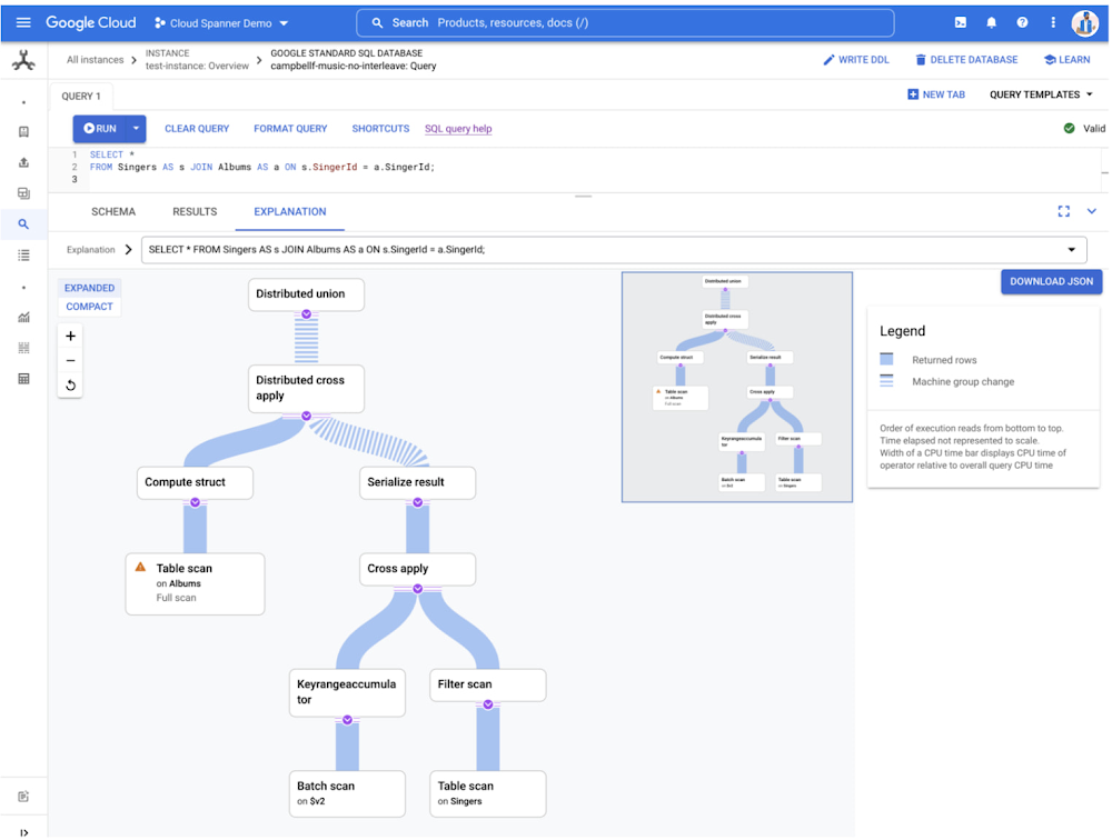
Spanner is a fully managed, distributed relational database that provides unlimited scale, global consistency, and up to five 9s availability. It was originally built to address Google’s needs to scale out Online Transaction Processing (OLTP) workloads without losing the benefits of strong consistency and familiar SQL that developers rely on. Today, Cloud Spanner is used in financial services, gaming, retail, health care, and other industries to power mission-critical workloads that need to scale without downtime. Like most modern relational databases, Spanner uses a query optimizer to find efficient execution plans for SQL queries. When a developer or a DBA writes a query in SQL, they describe the results they want to see, rather than how to access or update the data. This declarative approach allows the database to select different query plans depending on a wide variety of signals, such as the size and shape of the data and available indexes. Using these inputs, the query optimizer finds an execution plan for each query.You can see a graphical view of a plan from the Cloud Console. It shows the intermediate steps that Spanner uses to process the query. For each step, it details where time and resources are spent and how many rows each operation produces. This information is useful for identifying bottlenecks and to test changes to queries, indexes, or the query optimizer itself.How does the Spanner query optimizer work?Let’s start with the following example schema and query, using Spanner’s Google Standard SQL dialect. Schema:code_block[StructValue([(u’code’, u’CREATE TABLE Accounts (rn id STRING(MAX) NOT NULL,rn name STRING(MAX) NOT NULL,rn age INT64 NOT NULL,rn) PRIMARY KEY(id);rn rnCREATE INDEX AccountsByName ON Accounts(name);rn rnCREATE TABLE Orders (rn id STRING(MAX) NOT NULL,rn account_id STRING(MAX) NOT NULL,rn date DATE,rn total INT64 NOT NULL,rn) PRIMARY KEY(id);’), (u’language’, u”), (u’caption’, <wagtail.wagtailcore.rich_text.RichText object at 0x3e14c06e31d0>)])]Query:code_block[StructValue([(u’code’, u’SELECT a.id, o.order_idrnFROM Accounts AS a rnJOIN Orders AS o ON a.id = o.account_idrnWHERE a.name = “alice”rn AND o.date = “2022-1-1″;’), (u’language’, u”), (u’caption’, <wagtail.wagtailcore.rich_text.RichText object at 0x3e14ef462f90>)])]When Spanner receives a SQL query, it is parsed into an internal representation known as relational algebra. This is essentially a tree structure in which each node represents some operation of the original SQL. For example, every table access will appear as a leaf node in the tree and every join will be a binary node with its two inputs being the relations that it joins. The relational algebra for our example query looks like this:The query optimizer has two major stages that it uses to generate an efficient execution plan based on this relational algebra: heuristic optimization and cost-based optimization. Heuristic optimization, as the name indicates, applies heuristics, or pre-defined rules, to improve the plan. Those heuristics are manifested in several dozen replacement rules which are a subclass of algebraic transformation rule. Heuristic optimization improves the logical structure of the query in ways that are essentially guaranteed to make the query faster, such as moving filter operations closer to the data they filter, converting outer joins to inner joins where possible, and removing any redundancy in the query. However, many important decisions about an execution plan cannot be made heuristically, so they are made in the second stage, cost-based optimization, in which the query planner uses estimates of latency to choose between available alternatives. Let’s first look at how replacement rules work in heuristic optimization as a prelude to cost-based optimization.A replacement rule has two steps: a pattern matching step and an application step. In the pattern matching step, the rule attempts to match a fragment of the tree with some predefined pattern. When it finds a match, the second step is to replace the matched fragment of the tree with some other predefined fragment of tree. The next section provides a straightforward example of a replacement rule in which a filter operation is moved, or pushed, beneath a join.Example of a replacement ruleThis rule pushes a filer operation closer to the data that it is filtering. The rationale for doing this is two-fold: Pushing filters closer to the relevant data reduces the volume of data to be processed later in the pipelinePlacing a filter closer to the table creates an opportunity to use an index on the filtered column(s) to scan only the rows that qualify the filter.The rule matches the pattern of a filter node with a join node as its child. Details such as table names and the specifics of the filter condition are not part of the pattern matching. The essential elements of the pattern are just the filter with the join beneath it, the two shaded nodes in the tree illustrated below. The two leaf nodes in the picture need not actually be leaf nodes in the real tree, they themselves could be joins or other operations. They are included in the illustration simply to show context.The replacement rule rearranges the tree, as shown below, replacing the filter and join nodes. This changes how the query is executed, but does not change the results. The original filter node is split in two, with each predicate pushed to the relevant sides of the join from which the referenced columns are produced. This tells the query execution to filter the rows before they’re joined, so the join doesn’t have to handle rows that would later be rejected.Cost-based optimizationThere are big decisions about an execution plan for which no effective heuristics exist. These decisions must be made with an understanding of how different alternatives will perform. Hence the second stage of the query optimizer is the cost-based optimizer. In this stage, the optimizer makes decisions based on estimates of the latencies, or the costs, of different alternatives. Cost-based optimization provides a more dynamic approach than heuristics alone. It uses the size and shape of the data to calculate multiple execution plans. To developers, this means more efficient plans out-of-the-box and less hand tuning. The architectural backbone of this stage is the extensible optimizer generator framework known as Cascades. Cascades is the foundation of multiple industry and open-source query optimizers. This optimization stage is where the more impactful decisions are made, such as which indexes to use, what join order to use, and what join algorithms to use. Cost-based optimization in Spanner uses several dozen algebraic transformation rules. However, rather than being replacement rules, they are exploration and implementation rules. These classes of rules have two steps. As for replacement rules, the first step is a pattern matching step. However, rather than replacing the original matched fragment with some fixed alternative fragment, in general they provide multiple alternatives to the original fragment. Example of an exploration ruleThe following exploration rule matches a very simple pattern, a join. It generates one additional alternative in which the inputs to the join have been swapped. Such a transformation doesn’t change the meaning of the query because relational joins are commutative, in much the same way that arithmetic addition is commutative. The content of unshaded nodes in the following illustration do not matter to the rule and they are shown only to provide context.The following tree shows the new fragment that is generated. Specifically, the shaded node below is created as an available alternative to the original shaded node. It does not replace the original node. The unshaded nodes have swapped positions in the new alternative but are not modified in any way. They now have two parents instead of one. At this point, the query is no longer represented as a simple tree but as a directed acyclic graph (DAG). The rationale for this transformation is that the ordering of the inputs to a join can profoundly impact its performance. Typically, a join will perform faster if the first input that it accesses, which for Spanner means left side, is the smaller one. However, the optimal choice will also depend on many other factors, including the available indexes and the ordering requirements of the query.Example of an implementation ruleOnce again the following implementation rule pattern matches a join but this time it generates two alternatives: apply join and hash join. These two alternatives replace the original logical join operation.The above fragment will be replaced by the following two alternatives which are two possible ways of executing a join.Cascades and the evaluation engineThe Cascades engine manages the application of the exploration and implementation rules and all the alternatives they generate. It calls an evaluation engine to estimate the latency of fragments of execution plans and, ultimately, complete execution plans. The final plan that it selects is the plan with the lowest total estimated latency according to the evaluation engine. The optimizer considers many factors when estimating the latency of a node in an execution plan. These include exactly what operation the node performs (e.g. hash join, sort etc.), the storage medium when accessing data, and how the data is partitioned. But chief among those factors is an estimate of how many rows will enter the node and how many rows will exit the node. To estimate those row counts Spanner uses built-in statistics that characterize the actual data.Why does the query optimizer need statistics?How does the query optimizer select which strategies to use in assembling the plan? One important signal is descriptive statistics about the size, shape, and cardinality of the data. As part of regular operation, Spanner periodically samples each database to estimate metrics like distinct values, distributions of values, number of NULLs, data size for each column, and some combination of columns. These metrics are called optimizer statistics.To demonstrate how statistics help the optimizer pick a query plan, let’s consider a simple example using the previously described schema. Let’s look at the optimal plan for this query:code_block[StructValue([(u’code’, u’SELECT id, age FROM Accounts WHERE name = @p’), (u’language’, u”), (u’caption’, <wagtail.wagtailcore.rich_text.RichText object at 0x3e14edfdcf10>)])]There are two possible execution strategies that the query optimizer will consider:Base table plan: read all rows from Accounts and filter out those whose name is different from the value of parameter, @p.Index plan: Read the rows of accounts where name is equal to @p from the AccountsByName index. Then join the set with the Accounts table to fetch the age column.Let’s compare these visually in the plan viewer:Interestingly, even for this simple example there is no query plan that is obviously best. The optimal query plan depends on filter selectivity, or how many rows in Accounts match the condition. For the sake of simplicity let’s suppose that 10 rows in Accounts have name = “alice”, while the remaining 45,000 rows have name = “bob”. The latency of the query with each plan might look something like, using the fastest index plan for alice as our baseline:We can see in this simple example that the optimal query plan choice depends on the actual data stored in the database and the specific conditions in the query, in this example, up to 175 times faster. The statistics describe the shape of data in the database and help Spanner estimate which plan would be preferable for the query.Optimizer statistics collectionSpanner automatically updates the optimizer statistics to reflect the changes to the database schema and data. A background process recalculates them roughly every three days. The query optimizer will automatically use the latest version as input to query planning.In addition to automatic collection, you can also manually refresh the optimizer statistics using the ANALYZE DDL statement. This is particularly useful when a database’s schema or data are changing frequently, such as in a development environment, where you’re changing tables or indexes, or in production when large amounts of data are changing, such as in a new product launch or a large data clean-up. The optimizer statistics include:Approximate number of rows in each table.Approximate number of distinct values of each column and each composite key prefix (including index keys). For example if we have table T with key {a, b, c}, Spanner will store the number of distinct values for {a}, {a, b} and {a, b, c}.Approximate number of NULL, empty and NaN values in each column.Approximate minimum, maximum and average value byte size for each column.Histogram describing data distribution in each column. The histogram captures both ranges of values and frequent values.For example the Accounts table in the previous example has 45,010 total rows. The id column has 45,010 distinct values (since it is a key) and the name column has 2 distinct values (“alice” and “bob”).Histograms store a small sample of the column data to denote the boundaries of histogram bins. Disabling garbage collection for a statistics package will delay wipeout of this data. Query optimizer versioningThe Spanner development team is continuously improving the query optimizer. Each update broadens the class of queries where the optimizer picks the more efficient execution plan. The log of optimizer updates is available in the public documentation.We are doing extensive testing to ensure that new query optimizer versions select better query plans than before. Because of this, most workloads should not have to worry about query optimizer rollouts. By staying current they automatically inherit improvements as we enable them.There is a small chance, however, that an optimizer update will flip a query plan to a less performant one. If this happens, it will show up as a latency increase for the workload. Cloud Spanner provides several tools for customers to address this risk.Spanner users can choose which optimizer version to use for their queries. Databases use the newest optimizer by default. Spanner allows users to override the default query optimizer version through database options or set the desired optimizer version for each individual query.New optimizer versions are released as off-by-default for at least 30 days. You can track optimizer releases in the public Spanner release notes. After that, the new optimizer version is enabled by default. This period offers an opportunity to test queries against the new version to detect any regressions. In the rare cases that the new optimizer version selects suboptimal plans for critical SQL queries, you should use query hints to guide the optimizer. You can also pin a database or an individual query to the older query optimizer, allowing you to use older plans for specific queries, while still taking advantage of the latest optimizer for most queries. Pinning optimizer and statistics versions allows you to ensure plan stability to predictably rollout changes.In Spanner the query plan will not change as long the queries are configured to use the same optimizer version and rely on the same optimizer statistics. Users wishing to ensure that execution plans for their queries do not change can pin both the optimizer version and the optimizer statistics.To pin all queries against a database to an older optimizer version (e.g. version 4), you can set a database option via DDL:code_block[StructValue([(u’code’, u’ALTER DATABASE MyDatabase SET OPTIONS (optimizer_version = 4);’), (u’language’, u”), (u’caption’, <wagtail.wagtailcore.rich_text.RichText object at 0x3e14edff4350>)])]Spanner also provides a hint to more surgically pin a specific query. For example:code_block[StructValue([(u’code’, u’@{OPTIMIZER_VERSION=4} SELECT * FROM Accounts;’), (u’language’, u”), (u’caption’, <wagtail.wagtailcore.rich_text.RichText object at 0x3e14b7cf5fd0>)])]The Spanner documentation provides detailed strategies for managing the query optimizer version. Optimizer statistics versioningIn addition to controlling the version of the query optimizer, Spanner users can also choose which optimizer statistics will be used for the optimizer cost model. Spanner stores the last 30 days worth of optimizer statistics packages. Similarly to the optimizer version, the latest statistics package is used by default, and users can change it at a database or query level.Users can list the available statistics packages with this SQL query:code_block[StructValue([(u’code’, u’SELECT * FROM INFORMATION_SCHEMA.SPANNER_STATISTICS’), (u’language’, u”), (u’caption’, <wagtail.wagtailcore.rich_text.RichText object at 0x3e14b7cf54d0>)])]To use a particular statistics package it first needs to be excluded from garbage collection.code_block[StructValue([(u’code’, u’ALTER STATISTICS <package_name> SET OPTIONS (allow_gc=false);’), (u’language’, u”), (u’caption’, <wagtail.wagtailcore.rich_text.RichText object at 0x3e14ec3b7d50>)])]Then to use the statistics package by default for all queries against a database:code_block[StructValue([(u’code’, u’ALTER DATABASE <db>rnSET OPTIONS (optimizer_statistics_package = “<package name>”);’), (u’language’, u”), (u’caption’, <wagtail.wagtailcore.rich_text.RichText object at 0x3e14c01e5950>)])]Like the optimizer version above, you can also use a hint to pin the statistics package for an individual query using a hint:code_block[StructValue([(u’code’, u’@{OPTIMIZER_STATISTICS_PACKAGE=<package name>} SELECT * FROM Accounts;’), (u’language’, u”), (u’caption’, <wagtail.wagtailcore.rich_text.RichText object at 0x3e14c0f13b10>)])]Get started todayGoogle is continuously improving out-of-the-box performance of Spanner and reducing the need for manual tuning. The Spanner query optimizer uses multiple strategies to generate query plans that are efficient and performant. In addition to a variety of heuristics, Spanner uses true cost-based optimization to evaluate alternative plans and select the one with the lowest latency cost. To estimate these costs, Spanner automatically tracks statistics about the size and shape of the data, allowing the optimizer to adapt as schemas, indexes, and data change. To ensure plan stability, you can pin the optimizer version or the statistics that it uses at the database or query level. Learn more about the query optimizer or try out Spanner’s unmatched availability and consistency at any scale today for free for 90 days or as low as $65 USD per month.
Quelle: Google Cloud Platform

Building advanced Beam pipelines in Scala with SCIO

Apache Beam is an open source, unified programming model with a set of language-specific SDKs for defining and executing data processing workflows. Scio, pronounced shee-o, is Scala API for Beam developed by Spotify to build both Batch and Streaming pipelines. In this blog we will uncover the need for SCIO and a few reference patterns.Why ScioSCIO provides high level abstraction for developers and is preferred for following reasons:Striking balance between concise and performance. Pipeline written in Scala are concise compared to java with similar performanceEasier migration for Scalding/Spark developers due to similar semantics compared to Beam API thereby avoiding a steep learning curve for developers.Enables access to a large ecosystem of infrastructure libraries in Java e.g. Hadoop, Avro, Parquet and high level numerical processing libraries in Scala like Algebirdand Breeze.Supports Interactive exploration of data and code snippets using SCIO REPLReference Patterns Let us checkout few concepts along with examples: 1. Graph CompositionIf you have a complex pipeline consisting of several transforms, the feasible approach is to compose the logically related transforms into blocks.  This would make it easy to manage and debug the graph rendered on dataflow UI. Let us consider an example using popular WordCount pipeline. Fig:  Word Count Pipeline without Graph Composition Let us modify the code to group the related transforms into blocks:Fig:  Word Count Pipeline with Graph Composition2. Distributed CacheDistributed Cache allows to load the data from a given URI on workers and use the corresponding data across all tasks (DoFn’s) executing on the worker. Some of the common use cases are loading serialized machine learning model from object stores like Google Cloud Storage for running predictions,  lookup data references etc.Let us checkout an example that loads lookup data from CSV file on worker during initialization and utilizes to count the number of matching lookups for each input element.Fig:  Example demonstrating Distribute Cache3. Scio JoinsJoins in Beam are expressed using CoGroupByKey  while Scio allows to express various join types like inner, left outer and full outer joins through flattening the CoGbkResult. Hash joins (syntactic sugar over a beam side input) can be used, if one of the dataset is extremely small (max ~1GB) by representing a smaller dataset on the right hand side. Side inputs are small, in-memory data structures that are replicated to all workers and avoids shuffling. MultiJoin can be used to join up to 22 data sets. It is recommended that all data sets be ordered in descending size, because non-shuffle joins do require the largest data sets to be on the left of any chain of operators Sparse Joins can be used for cases where the left collection (LHS) is much larger than the right collection (RHS) that cannot fit in memory but contains a sparse intersection of keys matching with the left collection .  Sparse Joins are implemented by constructing a Bloom filter of keys from the right collection and split the left side collection into 2 partitions. Only the partition with keys in the filter go through the join and the rest are either concatenated (i.e Outer join) or discarded (Inner join). Sparse Join is especially useful for joining historical aggregates with incremental updates.Skewed Joins are a more appropriate choice for cases where the left collection (LHS) is much larger and contains hotkeys.  Skewed join uses Count Mink Sketch which is a probabilistic data structure to count the frequency of keys in the LHS collection.  LHS is partitioned into Hot and chill partitions.  While the Hot partition is joined with corresponding keys on RHS using a Hash join, chill partition uses a regular join and finally both the partitions are combined through union operation.Fig:  Example demonstrating Scio JoinsNote that while using Beam Java SDK you can also take advantage of some of the similar join abstractions using Join Library extension4. AlgeBird Aggregators and SemiGroupAlgebird is Twitter’s abstract algebra library containing several reusable modules for parallel aggregation and approximation. Algebird Aggregator or Semigroup can be used with aggregate and sum transforms on SCollection[T] or aggregateByKey and sumByKey transforms on SCollection[(K, V)].  Below example illustrates computing parallel aggregation on customer orders and composition of result into OrderMetrics classFig:  Example demonstrating Algebird Aggregators Below code snippet expands on previous example and demonstrates the SemiGroup for aggregation of objects by combining fields.Fig:  Example demonstrating Algebird SemiGroup5. GroupMap and GroupMapReduceGroupMap can be used as a replacement of groupBy(key) + mapValues(_.map(func)) or _.map(e  => kv.of(keyfunc, valuefunc)) + groupBy(key)Let us consider the below example that calculates the length of words for each type. Instead of grouping by each type and applying length function, the GroupMap allows combining these operations by applying keyfunc and valuefunc. Fig:  Example demonstrating GroupMapGroupMapReduce  can be used to derive the key and apply the associative operation on the values associated with each key. The associative function is performed locally on each mapper similarly to a “combiner” in MapReduce (aka combiner lifting) before sending the results to the reducer.  This is equivalent to keyBy(keyfunc) + reduceByKey(reducefunc) Let us consider the below example that calculates the cumulative sum of odd and even numbers in a given range.  In this case individual values are combined on each worker and the local results are aggregated to calculate the final resultFig:  Example demonstrating GroupMapReduceConclusionThanks for reading and I hope now you are motivated to learn more about SCIO.  Beyond the patterns covered above, SCIO contains several interesting features likeimplicit coders for Scala case classes,  Chaining jobs using I/O Taps , Distinct Count using HyperLogLog++ , Writing sorted output to files etc.  Several use case specific libraries like BigDiffy (comparison of large datasets) , FeaTran (used for ML Feature Engineering) were also built on top of SCIO. For Beam lovers with Scala background, SCIO is the perfect recipe for building complex distributed data pipelines.
Quelle: Google Cloud Platform

Built with BigQuery: How True Fit's data journey unlocks partner growth

Editor’s note: The post is part of a series highlighting our awesome partners, and their solutions, that are Built with BigQuery.“True Fit is in a unique position where we help shoppers find the right sizes of apparel and footwear through near real time, adaptable ML models thereby rendering a great shopping experience while also enabling retailers with higher conversion, revenue potential and more importantly access to actionable key business metrics. Our ability to process volumes of data, adapt our core ML models, reduce complex & slower ecosystems, exchange data easily with our customers etc, have been propelled multi-fold via BigQuery and Analytics Hub” – says Raj Chandrasekaran, CTO, True FitTrue Fit has built the world’s largest dataset for apparel and footwear retailers over the last twelve years, connecting purchasing and preference information for more than 80 million active shoppers to data for 17,000 brands across its global network of retail partners. This dataset powers fit personalization for shoppers as they buy apparel and footwear online and connects retailers with powerful data and insight to inform marketing, merchandising, product development and ecommerce strategy.Gathering data, correlating and analyzing it are the underlying foundation to making smart business decisions to grow and scale a retailer’s business. This is especially important for retailers that are utilizing data packages to target which consumers to market their brands and products to. Deriving meaningful insights from data has become a larger focus for retailers as the market grows digitally, competition for share of wallet increases and consumer expectations for more personalized  shopping experiences continues to rise.But, how do companies share datasets regardless of the magnitude amongst each other in a scalable manner by optimizing infrastructure costs and securely sharing data? How can companies access and use the data into their own environment without needing a complicated / time consuming process to physically move the data? How would a company know how to utilize this data to suit their own business needs? True Fit partnered with Google and the Built with BigQuery initiative to solve these questions.Google Cloud services such as BigQuery and Analytics Hub have become vital to how True Fit optimizes the entire lifecycle of data from ingestion to distribution of data packages with its retail partners. BigQuery is a fully managed, serverless and limitless scale data warehousing solution with tighter integration with several Google Cloud products. Analytics Hub, powered by BigQuery, allows easy creation of data exchanges for producers and simplifies the discovery and consumption of the data for the consumers. Data shared via the exchanges can further be enriched with more datasets available in the Analytics Hub marketplace.Using the above diagram, let us take a look at how the process works across different stages:Event Ingestion – True Fit leverages Cloud Logging with Fluentd to stream logging events into BigQuery as datasets. BigQuery’s unique capability in real time streaming allows for real time debugging and analysis of all activity across the True Fit ecosystem.Denormalization – Scheduled queries are set up to take the normalized data in the event logs and convert them into denormalized core tables. These tables are easy to query and contain all information needed to assist BI analysts and data scientists with their research without the need for complicated table joins.Aggregations – Aggregations are created and updated on the fly as data is ingested using a mix of scheduled queries and direct BigQuery table updates. Reports are always fresh and can be delivered without ever having to worry about stale data.Alerting – Alerts are set up all across the True Fit architecture which leverage the real-time aggregations. These alerts not only inform True Fit when there are data discrepancies or missing data but have also been configured to inform our partners when the data they provide contains errors. For example, True Fit will notify a retailer if the product catalog provided drops below specific thresholds we’ve previously seen from them. Alerts range from anything like an email, SMS message, or even a real-time toast message in a True Fit UI that a retailer is using to provide their data.Secure Distribution – Exchange’s are created in the Analytics Hub. The datasets are published as one or more listings into the Exchange. Partners subscribe to the listing as a linked dataset to get instant access to data and act upon it accordingly. This unlocks use cases that range from everywhere from marketing; to shopper chat bots; and even real-time product recommendations based on a shopper’s browsing behavior. Analytics Hub allows True Fit to expose only the data they intend to share to specific partners using simple to understand IAM roles. Adding the built-in Analytics Hub Subscriber role to a partner’s service account on a specific listing of dataset created just for them makes it so that they are the only one to get access to that data. Gone are the days of dealing with API keys or credential management!True Fit’s original data lake was built using Apache Hive prior to switching to BigQuery. At roughly 450TiB, extracting data from this data lake became quite a challenge to do in real-time. It took approximately 24 hours before data packages would become available to core retail partners which impacted our ability to produce reports and data packages at scale. Even after the data packages were available, partners had difficulty downloading these data packages and importing them into their own data warehouses to utilize due to the size and formats. The usefulness of the data packages would occasionally get put into question due to the data becoming stale and it was difficult to alert on any data discrepancies because of the time delay before these data packages would be available.BigQuery has allowed True Fit to produce these same data packages in real time as events occur; unlocking new marketing opportunities. Retail partners have also praised how easily consumable Analytics Hub has made the process because the data “just appears” alongside their existing data warehouse as linked datasets. True Fit publishes a number of BigQuery data packages for its retail partners via Analytics Hub which allows them to generate personalized onsite and email campaigns for their own shoppers in a manner far beyond the capabilities not available in the past. Below are just a sample of ways in which True Fit partners personalize their campaigns utilizing the True Fit data packages. Partners have the ability to:Find the True Fit shoppers of a desired category near real-time who’ve been browsing extra specific products in the last couple weeksEnhance their understanding of their shopper demographic data and category affinitiesRetrieve size and fit recommendations for specific in-stock products for a provided set of shoppers or have True Fit determine what the ideal set of shoppers for those products would beMatch their in-stock, limited run styles and sizes to applicable True Fit shoppersEnhance emails and on-site triggers based on products the shopper has recently viewed or purchased across the True Fit networkIf you’re a retailer looking to unlock your own growth using real-world data in real-time, be sure to check out the data packages offered by True Fit!To learn more about True Fit on Google Cloud, visit https://www.truefit.com/businessThe Built with BigQuery advantage for ISVs Through the Built with BigQuery Program launched in April ‘22 as part of the Google Data Cloud Summit, Google is helping data-driven companies like True Fit build innovative applications on Google’s data cloud with simplified access to technology, helpful and dedicated engineering support, and joint go-to-market programs. Participating companies can: Get started fast with a Google-funded, pre-configured sandbox. Accelerate product design and architecture through access to designated experts from the ISV Center of Excellence who can provide insight into key use cases, architectural patterns, and best practices. Amplify success with joint marketing programs to drive awareness, generate demand, and increase adoption.BigQuery gives ISVs the advantage of a powerful, highly scalable data warehouse that’s integrated with Google Cloud’s open, secure, sustainable platform. And with a huge partner ecosystem and support for multi-cloud, open source tools, and APIs, Google provides technology companies the portability and extensibility they need to avoid data lock-in.Click here to learn more about Built with BigQuery.We thank the many Google Cloud and True Fit team members who contributed to this ongoing collaboration and review, especially Raj Chandrasekaran, CTO True Fit and Sujit Khasnis, Cloud Partner Engineering
Quelle: Google Cloud Platform

Introducing Cloud Workstations: Managed and Secure Development environments in the cloud

With the unprecedented increase in remote collaboration over the last two years, development teams have had to find new ways to collaborate, driving increased demand for tools to address the productivity challenges of this new reality. This distributed way of working also introduces new security risks, such as data exfiltration — information leaving the company’s boundaries. For development teams, this means protecting the source code and data that serves as intellectual property for many companies. At Google Cloud Next, we introduced the public Preview of Cloud Workstations, which provides fully managed and integrated development environments on Google Cloud. Cloud Workstations is a solution focused on accelerating developer onboarding and increasing the productivity of developers’ daily workflows in a secure manner, and you can start using it today simply by visiting the Google Cloud console and configuring your first workstation.Cloud Workstations: Just the factsCloud Workstations provides managed development environments with built-in security, developer flexibility, and support for many popular developer tools. Cloud Workstations addressing the needs of enterprise technology teams.Developers can quickly access secure, fast, and customizable development environments anywhere, via a browser or from their local IDE. With Cloud Workstations, you can enforce consistent environment configurations, greatly reducing developer ramp-up time and addressing “works on my machine” problems.Administrators can easily provision, scale, manage, and secure development environments for their developers, providing them access to services and resources that are private, self-hosted, on-prem, or even running in other clouds. Cloud Workstations makes it easy to scale development environments, and helps automate everyday tasks, enabling greater efficiency and security.Cloud Workstations focuses on three core areas:Fast developer onboarding via consistent environmentsCustomizable development environmentsSecurity controls and policy supportFast developer onboarding via consistent environmentsGetting developers started on a new project can take days or weeks, with much of that time spent setting up the development environment. The traditional model of local setup may also lead to configuration drift over time, resulting in “works on my machine” issues that erode developer productivity and stifle collaboration.To address this, Cloud Workstations provides a fully managed solution for creating and managing development environments. Administrators or team leads can set up one or more workstation configurations as their teams’ environment templates. Updating or patching the environments of hundreds or thousands of developers is as simple as updating their workstation configuration and letting Cloud Workstations handle the updates.Developers can create their own workstations by simply selecting among the configurations to which they were granted access, making it easy to ensure consistency. When developers start writing code, they can be certain that they are using the right version of their tools.Customizable development environmentsDevelopers use a variety of tools and processes optimized to their needs. We designed Cloud Workstations to be flexible when it comes to tool choice, enabling developers to use the tools they’re the most productive with, while enjoying the benefits of remote development. Here are some of the capabilities that enable this flexibility:Multi-IDE support: Developers use different IDEs for different tasks, and often customize them for their maximum efficiency. Cloud Workstations supports multiple managed IDEs such as IntelliJ IDEA Ultimate, PyCharm Professional, GoLand, WebStorm, Rider, Code-OSS, and many more. We’ve also partnered with JetBrains so that you can bring your existing licenses to Cloud Workstations. These IDEs are provided via optimized browser-based or local-client interfaces, avoiding the latency and challenges of general-purpose remote desktop tools such as latency and limited customization.Container-based customization: Beyond IDEs, development environments also comprise libraries, IDE extensions, code samples, and even test databases and servers. To help ensure your developers are getting the tools they need quickly, you can extend the Cloud Workstations container images with the tools of your choice.Support for third-party DevOps tools: Every organization has its own tried and tested tools — Google Cloud services such as Cloud Build, but also third-party tools such as GitLab, TeamCity, or Jenkins. By running Cloud Workstations inside your Virtual Private Cloud (VPC), you can connect to tools self-hosted in Google Cloud, on-prem, or even in other clouds.Security controls and policy supportWith Cloud Workstations, you can extend the same security policies and mechanisms you use for your production services in the cloud to your developer workstations. Here are some of the ways that Cloud Workstations helps to ensure the security of your development environments:No source code or data is transferred or stored on local machines.Each workstation runs on a single dedicated virtual machine, for increased isolation between development environments.Identity and Access Management (IAM) policies are automatically applied, and follow the principle of least privilege, helping to limit workstation access to a single developer.Workstations can be created directly inside your project and VPC, allowing you to help enforce policies like firewall rules or scheduled disk backups.VPC Service Controls can be used to define a security perimeter around your workstations, constraining access to sensitive resources, and helping prevent data exfiltration.Environments can be automatically updated after a session reaches a time limit, so that developers automatically get any updates in a timely manner.Fully private ingress/egress is also supported, so that only users inside your private network can access your workstations.What customers and partners are saying”We have hundreds of developers all around the world that need to be able to be connected anytime, from any device. Cloud Workstations enabled us to replace our custom solution with a more secure, controlled and globally managed solution.” — Sebastien Morand, Head of Data Engineering, L’Oréal“With traditional full VDI solutions, you have to take care of the operating system and other factors which are separate from the developer experience. We are looking for a solution that solves problems without introducing new ones.” — Christian Gorke, Head of Cyber Center of Excellence, Commerzbank“We are incredibly excited to tightly partner with Google Cloud around their Cloud Workstations initiative, that will make remote development with JetBrains IDEs available to Google Cloud users worldwide. We look forward to working together on making developers more productive with remote development while improving security and saving computation resources.” — Max Shafirov, CEO, JetBrainsGet started todayTry Cloud Workstations today by visiting your console, or learn more on our webpage, in our documentation or by watching this Cloud Next session. Cloud Workstations is a key part of our end-to-end Software Delivery Shield offering. To learn more about Software Delivery Shield, visit this webpage.
Quelle: Google Cloud Platform