Krypto-Winter: Bitcoin-Kurs wächst im Januar stark
Im Januar ist der Kurs des Bitcoin um etwa 40 Prozent gestiegen. Von seinem Höchststand ist er aber weit entfernt. (Bitcoin, Börse)
Quelle: Golem

Im Januar ist der Kurs des Bitcoin um etwa 40 Prozent gestiegen. Von seinem Höchststand ist er aber weit entfernt. (Bitcoin, Börse)
Quelle: Golem

Amazons Entlassungswelle führt erstmal zu hohen Kosten: 640 Millionen US-Dollar sind für Abfindungen gezahlt worden. (Amazon, Börse)
Quelle: Golem

Trotz Umsatzsteigerung ist der Gewinn von Alphabet kleiner ausgefallen. Google kündigt einen ChatGPT-Konkurrenten an. (Alphabet, Google)
Quelle: Golem

Das Redmagic 8 Pro ist eines der ersten Smartphones mit Qualcomms Snapdragon 8 Gen2. Das Gerät hat eine hohe Leistung, ist aber nicht perfekt. Ein Test von Tobias Költzsch (Smartphone, Android)
Quelle: Golem

Nicht nur Nutzer, sondern auch Entwickler sollen zukünftig bezahlen: Twitter macht den API-Zugang kostenpflichtig (Twitter, API)
Quelle: Golem

Quelle: <a href="RIP To The Best Bots On Twitter“>BuzzFeed

Quelle: <a href="Inside Virtual Reality's Booming Underground Sex Scene“>BuzzFeed
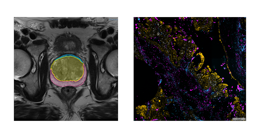
Medical imaging offers remarkable opportunities in research for advancing our understanding of cancer, discovering new non-invasive methods for its detection, and improving overall patient care. Advancements in artificial intelligence (AI), in particular, have been key in unlocking our ability to use this imaging data as part of cancer research. Development of AI-powered research approaches, however, requires access to large quantities of high quality imaging data. Sample images from NCI Imaging Data Commons. Left: Magnetic Resonance Imaging (MRI) of the prostate (credit: http://doi.org/10.7937/K9/TCIA.2018.MR1CKGND), along with the annotations of the prostate gland and substructures. Right: highly-multiplexed fluorescence tissue imaging of melanoma (credit: https://humantumoratlas.org/hta7/).The US National Cancer Institute (NCI) has long prioritized collection, curation, and dissemination of comprehensive, publicly available cancer imaging datasets. Initiatives like The Cancer Genome Atlas (TCGA) and Human Tumor Atlas Network (HTAN) (to name a few) work to make robust, standardized datasets easily accessible to anyone interested in contributing their expertise: students learning the basics of AI, engineers developing commercial AI products, researchers developing innovative proposals for image analysis, and of course the funders evaluating those proposals.Even so, there continue to be challenges that complicate sharing and analysis of imaging data:Data is spread across a variety of repositories, which means replicating data to bring it together or within reach of tooling (such as cloud-based resources).Images are often stored in vendor-specific or specialized research formats which complicates analysis workflows and increases maintenance costs.Lack of a common data model or tooling make capabilities such as search, visualization, and analysis of data difficult and repository- or dataset-specific. Achieving reproducibility of the analysis workflows, a critical function in research, is challenging and often lacking in practice.Introducing Imaging Data CommonsTo address these issues, as part of the Cancer Research Data Commons (CRDC) initiative that establishes the national cancer research ecosystem, NCI launched the Imaging Data Commons (IDC), a cloud-based repository of publicly available cancer imaging data with several key advantages:Colocation: Image files are curated into Google Cloud Storage buckets, side-by-side with on-demand computational resources and cloud-based tools, making it easier and faster for you to access and analyze.Format: Images, annotations and analysis results are harmonized into the standard DICOM (Data Imaging and Communications and Medicine) format to improve interoperability with tools and support uniform processing pipelines.Tooling: IDC maintains tools that – without having to download anything – allow you to explore and search the data, and visualize images and annotations. You can easily access IDC data from the cloud-based tools available in Google Cloud, such as Vertex AI, Colab, or deploy your own tools in highly configurable virtual environments.Reproducibility: Sharing reproducible analysis workflows is streamlined through maintaining persistent versioned data that you can use to precisely define cohorts used to train or validate algorithms, which in turn can be deployed in virtual environments that can provide consistent software and hardware configuration.IDC ingests and harmonizes de-identified data from a growing list of repositories and initiatives, spanning a broad range of image types and scales, cancer types, and manufacturers. A significant portion of these images are accompanied by annotations and clinical data. For a quick summary of what is available in IDC, check the IDC Portal or this Looker Studio dashboard! Exploring the IDC dataIDC PortalA great place to start exploring the data is the IDC Portal. From this in-browser portal, you can use some of the key metadata attributes to navigate the images and visualize them.Navigating the IDC portal to view dataset imagesAs an example, here are the steps you can follow to find slide microscopy images for patients with lung cancer:From the IDC Portal, proceed to “Explore images”.In the top right portion of the exploration screen, use the summary pie chart to select Chest primary site (you could alternatively select Lung, noting that annotation of cancer location can use different terms).In the same pie chart summary section, navigate to Modality and select Slide Microscopy.In the right-hand panel, scroll to the Collections section, which will now list all collections containing relevant images. Select one or more collections using the checkboxes. Navigate to the Selected Cases section just below, where you will find a list of patients within the selected collections that meet the search criteria. Next, select a given patient using the checkbox. Navigating to the Selected Studies section just below will now show the list of studies – think of these as specific imaging exams available for this patient. Click the “eye” icon on the far right which will open the viewer allowing you to see the images themselves.BigQuery Public DatasetWhen it’s time to search and select the subsets (or cohorts) of the data that you need to support your analysis more precisely, you’ll head to the public dataset in BigQuery. This dataset contains the comprehensive set of metadata available for the IDC images (beyond the subset contained in the IDC portal), which you can use to precisely define your target data subset with a custom, standard SQL query.You can run these queries from the in-browser BigQuery Console by creating a BigQuery sandbox. The BigQuery sandbox enables you to query data within the limits of the Google Cloud free tier without needing a credit card. If you decide to enable billing and go above the free tier threshold, you are subject to regular BigQuery pricing. However, we expect most researchers’ needs will fit within this tier. To get started with an exploratory query, you can select studies corresponding to the same criteria you just used in your exploration of the IDC Portal:code_block[StructValue([(u’code’, u’SELECTrn DISTINCT(StudyInstanceUID)rnFROMrn `bigquery-public-data.idc_current.dicom_all`rnWHERErn tcia_tumorLocation = “Chest”rn AND Modality = “SM”‘), (u’language’, u’lang-sql’), (u’caption’, <wagtail.wagtailcore.rich_text.RichText object at 0x3e11af929610>)])]Alright now you’re ready to write a query that creates precisely defined cohorts. This time we’ll shift from exploring digital pathology images to subsetting Computed Tomography (CT) scans that meet certain criteria.The following query selects all files, identified by their unique storage path in the gcs_url column, and corresponding to CT series that have SliceThickness between 0 and 1 mm. It also builds a URL in series_viewer_url that you can follow to visualize the series in the IDC Portal viewer. For the sake of this example, the results are limited to only one series.code_block[StructValue([(u’code’, u’SELECTrn collection_id,rn PatientID,rn SeriesDescription,rn SliceThickness,rn gcs_url,rn CONCAT(“https://viewer.imaging.datacommons.cancer.gov/viewer/”,StudyInstanceUID, “?seriesInstanceUID=”, SeriesInstanceUID) AS series_viewer_urlrnFROMrn `bigquery-public-data.idc_current.dicom_all`rnWHERErn SeriesInstanceUID IN (rn SELECTrn SeriesInstanceUIDrn FROMrn `bigquery-public-data.idc_current.dicom_all`rn WHERErn Modality = “CT”rn AND SAFE_CAST(SliceThickness AS FLOAT64) > 0rn AND SAFE_CAST(SliceThickness AS FLOAT64) < 1rn LIMITrn 1)’), (u’language’, u’lang-sql’), (u’caption’, <wagtail.wagtailcore.rich_text.RichText object at 0x3e11af3287d0>)])]As you start to write more complex queries, it will be important to familiarize yourself with the DICOM format, and how it is connected with the IDC dataset. This getting started tutorial is a great place to start learning more.What can you do with the results of these queries? For example:You can build the URL to open the IDC Portal viewer and examine individual studies, as we demonstrated in the second query above.You can learn more about the patients and studies that meet this search criteria by exploring what annotations or clinical data available accompanying these images. The getting started tutorial provides several example queries along these lines.You can link DICOM metadata describing imaging collections with related clinical information, which is linked when available. This notebook can help in navigating clinical data available for IDC collections.Finally, you can download all images contained in the resulting studies. Thanks to the support of Google Cloud Public Dataset Program, you are able to download IDC image files from Cloud Storage without cost.Integrating with other Cloud toolsThere are several Cloud tools we want to mention that can help in your explorations of the IDC data:Colab: Colab is a hosted Jupyter notebook solution that allows you to write and share notebooks that combine text and code, download images from IDC, and execute the code in the cloud with a free virtual machine. You can expand beyond the free tier to use custom VMs or GPUs, while still controlling costs with fixed monthly pricing plans. Notebooks can easily be shared with colleagues (such as readers of your academic manuscript). Check out these example Colab notebooks to help you get started.Vertex AI: Vertex AI is a platform to handle all the steps of the ML workflow. Again, it includes managed Jupyter notebooks, but with more control over the environment and hardware you use. As part of Google Cloud, it also comes with enterprise-grade security, which may be important to your use case, especially if you are joining in your own proprietary data. Its Experiments functionality allows you to automatically track architectures, hyperparameters, and training environments, to help you discover the optimal ML model faster. Looker Studio: Looker Studio is a platform for developing and sharing custom interactive dashboards. You can create dashboards that are focused on a specific subset of metadata accompanying the images and cater to the users that prefer interactive interface over the SQL queries. As an example, this dashboard provides a summary of IDC data, and this dashboard focuses on the preclinical datasets within the IDC.Cloud Healthcare API: IDC relies on Cloud Healthcare API to extract and manage DICOM metadata with BigQuery, and to maintain DICOM stores that make IDC data available via the standard DICOMweb interface. IDC users can utilize these tools to store and provide access to the artifacts resulting from the analysis of IDC images. As an example, DICOM store can be populated with the results of image segmentation, which could be visualized using a user-deployed Firebase-hosted instance of OHIF Viewer (deployment instructions are available here).Next StepsThe IDC dataset is a powerful tool for accelerating data-driven research and scientific discovery in cancer prevention, treatment, and diagnosis. We encourage researchers, engineers, and students alike to get started by following the onboarding steps we laid out in this post: familiar yourselves with the data by heading to the IDC portal, tailor your cohorts using the BigQuery public dataset, and then download the images to analyze with your on-prem tools, or with Google Cloud services or Colab. Getting started with the IDC notebook series should help you get familiar with the resource.For questions, you can reach the IDC team at support@canceridc.dev, or join the IDC community and post your questions. Also, see the IDC user guide for more details, including official documentation.Related ArticleBoost medical discoveries with AlphaFold on Vertex AILearn 3 ways to run AlphaFold on Google Cloud using no-cost solutions and guides.Read ArticleRelated ArticleMost popular public datasets to enrich your BigQuery analysesCheck out free public datasets from Google Cloud, available to help you get started easily with big data analytics in BigQuery and Cloud …Read Article
Quelle: Google Cloud Platform
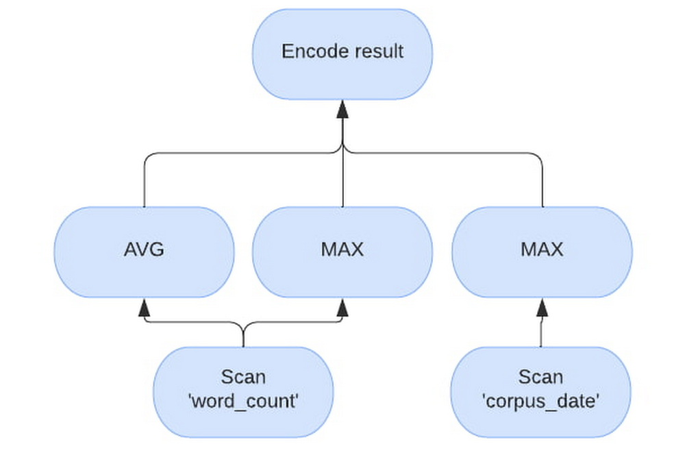
BigQuery BI Engine is a fast, in-memory analysis system for BigQuery currently processing over 2 billion queries per month and growing. BigQuery has its roots in Google’s Dremel system and is a data warehouse built with scalability as a goal. On the other hand BI Engine was envisioned with data analysts in mind and focuses on providing value on Gigabyte to sub-Terabyte datasets, with minimal tuning, for real time analytics and BI purposes.Using BI Engine is simple – create a memory reservation on the project that runs BigQuery queries, and it will cache data and use the optimizations. This post is a deep dive into how BI Engine helps deliver blazing fast performance for your BigQuery queries and what users can do to leverage its full potential. BI Engine optimizationsThe two main pillars of BI Engine are in-memory caching of data and vectorized processing. Other optimizations include CMETA metadata pruning, single-node processing, and join optimizations for smaller tables.Vectorized engineBI Engine utilizes the “Superluminal” vectorized evaluation engine which is also used for YouTube’s analytic data platform query engine – Procella. In BigQuery’s row-based evaluation, the engine will process all columns within a row for every row. The engine is potentially alternating between column types and memory locations before going to the next row. In contrast, a vectorized engine like Superluminal will process a block of values of the same type from a single column for as long as possible and only switch to the next column when necessary. This way, hardware can run multiple operations at once using SIMD, reducing both latency and infrastructure costs. BI Engine dynamically chooses block size to fit into caches and available memory.For the example query, “SELECT AVG(word_count), MAX(word_count), MAX(corpus_date) FROM samples.shakespeare”, will have the following vectorized plan. Note how the evaluation processes “word_count” separately from “corpus_date”.In-memory cacheBigQuery is a disaggregated storage and compute engine. Usually the data in BigQuery is stored on Google’s distributed file system – Colossus, most often in blocks in Capacitor format and the compute is represented by Borg tasks. This enables BigQuery’s scaling properties. To get the most out of vectorized processing, BI Engine needs to feed the raw data at CPU speeds, which is achievable only if the data is already in memory. BI Engine runs Borg tasks as well, but workers are more memory-heavy to be able to cache the data as it is being read from Colossus.A single BigQuery query can be either sent to a single BI Engine worker, or sharded and sent to multiple BI Engine workers. Each worker receives a piece of a query to execute with a set of columns and rows necessary to answer it. If the data is not cached in the workers memory from the previous query, the worker loads the data from Colossus into local RAM. Subsequent requests for the same or subset of columns and rows are served from memory only. Note that workers will unload the contents if data hasn’t been used for over 24 hours. As multiple queries arrive, sometimes they might require more CPU time than available on a worker, if there is still reservation available, a new worker will be assigned to same blocks and subsequent requests for the same blocks will be load-balanced between the workers.BI Engine can also process super-fresh data that was streamed to the BigQuery table. Therefore, there are two formats supported by BI Engine workers currently – Capacitor and streaming. In-memory capacitor blocksGenerally, data in a capacitor block is heavily pre-processed and compressed during generation. There are a number of different ways the data from the capacitor block can be cached, some are more memory efficient, while others are more CPU efficient. BI Engine worker intelligently chooses between those preferring latency and CPU-efficient formats where possible. Thus actual reservation memory usage might not be the same as logical or physical storage usage due to the different caching formats.In-memory streaming dataStreaming data is stored in memory as blocks of native array-columns and is lazily unloaded when blocks get extracted into Capacitor by underlying storage processes. Note that for streaming, BI workers need to either go to streaming storage every time to potentially obtain new blocks or serve slightly stale data. BI Engine prefers serving slightly stale data and loading the new streaming blocks in the background instead.BI Engine worker does this opportunistically during the queries, if the worker detects streaming data and the cache is newer than 1 minute, a background refresh is launched in parallel with the query. In practice, this means that with enough requests the data is no more stale than the previous request time. For example if a request arrives every second, then the streaming data will be around a second stale.First requests loading data are slowDue to the read time optimizations, loading data from previously unseen columns can take longer than BigQuery does. Subsequent reads will benefit from these optimizations.For example, the query above here is backend time for a sample run of the same query with BI Engine off, first run and subsequent run.Multiple block processing and dynamic single worker executionBI Engine workers are optimized for BI workloads where the output size will be small compared to the input size and the output will be mostly aggregated. In regular BigQuery execution, a single worker tries to minimize data loading due to network bandwidth limitations. Instead, BigQuery relies on massive parallelism to complete queries quickly. On the other hand, BI Engine prefers to process more data in parallel on a single machine. If the data has been cached, there is no network bandwidth limitation and BI Engine further reduces network utilization by reducing the number of intermediate “shuffle” layers between query stages.With small enough inputs and a simple query, the entire query will be executed on a single worker and the query plan will have a single stage for the whole processing. We constantly work on making more tables and query shapes eligible for a single stage processing, as this is a very promising way to improve the latency of typical BI queries.For the example query, which is very simple and the table is very small, here is a sample run of the same query with BI Engine distributed execution vs single node (default).How to get most out of BI EngineWhile we all want a switch that we can toggle and everything becomes fast, there are still some best practices to think about when using BI Engine.Output data sizeBI optimizations assume human eyes on the other side and that the size of output data is small enough to be comprehensible by a human. This limited output size is achieved by selective filters and aggregations. As a corollary, instead of SELECT * (even with a LIMIT), a better approach will be to provide the fields one is interested in with an appropriate filter and aggregation.To show this on an example – query “SELECT * FROM samples.shakespeare” processes about 6MB and takes over a second with both BigQuery and BI Engine. If we add MAX to every field – “SELECT MAX(word), MAX(word_count), MAX(corpus), MAX(corpus_date) FROM samples.shakespeare”, both engines will read all of the data, perform some simple comparisons and finish 5 times faster on BigQuery and 50 times faster on BI Engine.Help BigQuery with organizing your dataBI Engine uses query filters to narrow down the set of blocks to read. Therefore, partitioning and clustering your data will reduce the amount of data to read, latency and slot usage. With a caveat, that “over partitioning” or having too many partitions might interfere with BI Engine multi-block processing. For optimal BigQuery and BI Engine performance, partitions larger than one gigabyte are preferred.Query depthBI Engine currently accelerates stages of the query that read data from the table, which are typically the leaves of the query execution tree. What this means in practice is that almost every query will use some BigQuery slots.That’s why one gets the most speedup from BI Engine when a lot of time is spent on leaf stages. To mitigate this, BI Engine tries to push as many computations as possible to the first stage. Ideally, execute them on a single worker, where the tree is just one node.For example Query1 of TPCH 10G benchmark, is relatively simple. It is 3 stages deep with efficient filters and aggregations that processes 30 million rows, but outputs just 1.Running this query in BI Engine we see that the full query took 215 ms with “S00: Input” stage being the one accelerated by BI Engine taking 26 ms.Running the same query in BigQuery gets us 583ms, with “S00: Input” taking 229 ms.What we see here is that the “S00: Input” stage run time went down 8x, but the overall query did not get 8x faster, as the other two stages were not accelerated and their run time remained roughly the same. With breakdown between stages illustrated by the following figure.In a perfect world, where BI Engine processes its part in 0 milliseconds, the query will still take 189ms to complete. So the maximum speed gain for this query is about 2-3x. If we, for example, make this query heavier on the first stage, by running TPCH 100G instead, we see that BI Engine finishes the query 6x faster than BigQuery, while the first stage is 30 times faster!vs 1 second on BigQueryOver time, our goal is to expand the eligible query and data shapes and collapse as many operations as feasible into a single BI Engine stage to realize maximum gains.JoinsAs previously noted, BI Engine accelerates “leaf” stages of the query. However, there is one very common pattern used in BI tools that BI Engine optimizes. It’s when one large “fact” table is joined with one or more smaller “dimension” tables. Then BI Engine can perform multiple joins, all in one leaf stage, using so-called “broadcast” join execution strategy.During the broadcast join, the fact table is sharded to be executed in parallel on multiple nodes, while the dimension tables are read on each node in their entirety.For example, let’s run Query 3 from the TPC-DS 1G benchmark. The fact table is store_sales and the dimension tables are date_dim and item. In BigQuery the dimension tables will be loaded into shuffle first, then the “S03: Join+” stage will, for every parallel part of store_sales, read all necessary columns of two dimension tables, in their entirety, to join.Note that filters on date_dim and item are very efficient, and the 2.9M row fact table is joined only with about 6000 rows. BI Engine plan will look a bit different, as BI Engine will cache the dimension tables directly, but the same principle applies. For BI Engine, let’s assume that two nodes will process the query due to the store_sales table being too big for a single node processing. We can see on the image below that both nodes will have similar operations – reading the data, filtering, building the lookup table and then performing the join. While only a subset of data for the store_sales table is being processed on each, all operations on dimension tables are repeated.Note that”build lookup table” operation is very CPU intensive compared to filtering”join” operation performance also suffers if the lookup tables are large, as it interferes with CPU cache localitydimension tables need to be replicated to each “block” of fact tableThe takeaway is when join is performed by BI Engine, the fact table is sometimes split into different nodes. All other tables will be copied multiple times on every node to perform the join. Keeping dimension tables small or selective filters will help to make sure join performance is optimal.ConclusionsSummarizing everything above, there are some things one can do to make full use of BI Engine and make their queries fasterLess is more when it comes to data returned – make sure to filter and aggregate as much data as possible early in the query. Push down filters and computations into BI Engine.Queries with a small number of stages get the best acceleration. Preprocessing the data to minimize query complexity will help with optimal performance. For example, using materialized views can be a good option.Joins are sometimes expensive, but BI Engine may be very efficient in optimizing typical star schema queries.It’s beneficial to partition and/or cluster the tables to limit the amount of data to be read.Special thanks to Benjamin Liles, Software Engineer for BI Engine, Deepak Dayama, Product Manager for BI Engine, for contributing to this post.
Quelle: Google Cloud Platform

This post was co-authored by Suren Jamiyanaa, Product Manager II, Azure Networking.
As large organizations across all industries expand their cloud business and operations, one core criteria for their cloud infrastructure is to make connections over the internet at scale. However, a common outbound connectivity issue encountered when handling large-scale outbound traffic is source network address translation (SNAT) port exhaustion. Each time a new connection to the same destination endpoint is made over the internet, a new SNAT port is used. SNAT port exhaustion occurs when all available SNAT ports run out. Environments that often require making many connections to the same destination, such as accessing a database hosted in a service provider’s data center, are susceptible to SNAT port exhaustion. When it comes to connecting outbound to the internet, customers need to not only consider potential risks such as SNAT port exhaustion but also how to provide security for their outbound traffic.
Azure Firewall is an intelligent security service that protects cloud infrastructures against new and emerging attacks by filtering network traffic. All outbound internet traffic using Azure Firewall is inspected, secured, and undergoes SNAT to conceal the original client IP address. To bolster outbound connectivity, Azure Firewall can be scaled out by associating multiple public IPs to Azure Firewall. Some large-scale environments may require manually associating up to hundreds of public IPs to Firewall in order to meet the demand of large-scale workloads, which can be a challenge to manage long-term. Partner destinations also commonly have a limit on the number of IPs that can be whitelisted at their destination sites, which can create challenges when Firewall outbound connectivity needs to be scaled out with many public IPs. Without scaling this outbound connectivity, customers are more susceptible to outbound connectivity failures due to SNAT port exhaustion.
This is where network address translation (NAT) gateway comes in. NAT gateway can be easily deployed to an Azure Firewall subnet to automatically scale connections and filter traffic through the firewall before connecting to the internet. NAT gateway not only provides a larger SNAT port inventory with fewer public IPs but NAT gateway’s unique method of SNAT port allocation is specifically designed to handle dynamic and large-scale workloads. NAT gateway’s dynamic allocation and randomized selection of SNAT ports significantly reduce the risk of SNAT port exhaustion while also keeping overhead management of public IPs at a minimum.
In this blog, we’ll explore the benefits of using NAT Gateway with Azure Firewall as well as how to integrate both into your architecture to ensure you have the best setup for meeting your security and scalability needs for outbound connectivity.
Benefits of using NAT Gateway with Azure Firewall
One of the greatest benefits of integrating NAT gateway into your Firewall architecture is the scalability that it provides for outbound connectivity. SNAT ports are a key component to making new connections over the internet and distinguishing different connections from one another coming from the same source endpoint. NAT gateway provides 64,512 SNAT ports per public IP and can scale out to use 16 public IP addresses. This means, when fully scaled out with 16 public IP addresses, NAT gateway provides over 1 million SNAT ports. Azure Firewall, on the other hand, supports 2,496 SNAT ports per public IP per virtual machine instance within a virtual machine scale set (minimum of 2 instances). This means that to achieve the same volume of SNAT port inventory as NAT gateway when fully scaled out, Firewall may require up to 200 public IPs. Not only does NAT gateway offer more SNAT ports with fewer public IPs, but these SNAT ports are allocated on demand to any virtual machine in a subnet. On-demand SNAT port allocation is key to how NAT gateway significantly reduces the risk of common outbound connectivity issues like SNAT port exhaustion.
NAT gateway also provides 50 Gbps of data throughput for outbound traffic that can be used in line with a standard SKU Azure Firewall, which provides 30 Gbps of data throughput. Premium SKU Azure Firewall provides 100 Gbps of data throughput.
With NAT gateway you also ensure that your outbound traffic is entirely secure since no inbound traffic can get through NAT gateway. All inbound traffic is subject to security rules enabled on the Azure Firewall before it can reach any private resources within your cloud infrastructure.
To learn more about the other benefits that NAT gateway offers in Azure Firewall architectures, see NAT gateway integration with Azure Firewall.
How to get the most out of using NAT Gateway with Azure Firewall
Let’s take a look at how to set up NAT gateway with Azure Firewall and how connectivity to and from the internet works upon integrating both into your cloud architecture.
Production-ready outbound connectivity with NAT Gateway and Azure Firewall
For production workloads, Azure recommends separating Azure Firewall and production workloads into a hub and spoke topology. Introducing NAT gateway into this setup is simple and can be done in just a couple short steps. First, deploy Azure Firewall to an Azure Firewall Subnet within the hub virtual network (VNet). Attach NAT gateway to the Azure Firewall Subnet and add up to 16 public IP addresses and you’re done. Once configured, NAT gateway becomes the default route for all outbound traffic from the Azure Firewall Subnet. This means that internet-directed traffic (traffic with the prefix 0.0.0.0/0) routed from the spoke Vnets to the Hub Vnet’s Azure Firewall Subnet will automatically use the NAT gateway to connect outbound. Because NAT gateway is fully managed by Azure, NAT gateway allocates SNAT ports and scales to meet your outbound connectivity needs automatically. No additional configurations are required.
Figure: Separate the Azure Firewall from the production workloads in a hub and spoke topology and attach NAT gateway to the Azure Firewall Subnet in the hub virtual network. Once configured, all outbound traffic from your spoke virtual networks is directed through NAT gateway and all return traffic is directed back to the Azure Firewall Public IP to maintain flow symmetry.
How to set up NAT Gateway with Azure Firewall
To ensure that you have set up your workloads to route to the Azure Firewall Subnet and use NAT gateway for connecting outbound, follow these steps:
Deploy your Firewall to an Azure Firewall Subnet within its own virtual network. This will be the Hub Vnet.
Add NAT gateway to the Azure Firewall Subnet and attach at least one public IP address.
Deploy your workloads to subnets in separate virtual networks. These virtual networks will be the spokes. Create as many spoke Vnets for your workload as needed.
Set up Vnet peering between the hub and spoke Vnets.
Insert a route to the spoke subnets to route 0.0.0.0/0 internet traffic to the Azure Firewall.
Add a network rule to the Firewall policy to allow traffic from the spoke Vnets to the internet.
Refer to this tutorial for step-by step guidance on how to deploy NAT gateway and Azure Firewall in a hub and spoke topology.
Once NAT gateway is deployed to the Azure Firewall Subnet, all outbound traffic is directed through the NAT gateway. Normally, NAT gateway also receives any return traffic. However, in the presence of Azure Firewall, NAT gateway is used for outbound traffic only. All inbound and return traffic is directed through the Azure Firewall in order to ensure traffic flow symmetry.
FAQ
Can NAT gateway be used in a secure hub virtual network architecture with Azure Firewall?
No, NAT gateway is not supported in a secure hub (vWAN) architecture. A hub virtual network architecture as described above must be used instead.
How does NAT gateway work with a zone-redundant Azure Firewall?
NAT gateway is a zonal resource that can provide outbound connectivity from a single zone for a virtual network regardless of whether it used with a zonal or zone-redundant Azure Firewall. To learn more about how to optimize your availability zone deployments with NAT gateway, refer to our last blog.
Benefits of NAT Gateway with Azure Firewall
When it comes to providing outbound connectivity to the internet from cloud architectures using Azure Firewall, look no further than NAT gateway. The benefits of using NAT gateway with Azure Firewall include:
Simple configuration. Attach NAT gateway to the Azure Firewall Subnet in a matter of minutes and start connecting outbound right away. No additional configurations required.
Fully managed by Azure. NAT gateway is fully managed by Azure and automatically scales to meet the demand of your workload.
Requires fewer static public IPs. NAT gateway can be associated with up to 16 static public IP addresses which allows for easy whitelisting at destination endpoints and simpler management of downstream IP filtering rules.
Provides a greater volume of SNAT ports for connecting outbound. NAT gateway can scale to over 1 million SNAT ports when configured to 16 public IP addresses.
Dynamic SNAT port allocation ensures that the full inventory of SNAT ports is available to every virtual machine in your workload. This in turn helps to significantly reduce the risk of SNAT port exhaustion that is common with other SNAT methods.
Secure outbound connectivity. Ensures that no inbound traffic from the internet can reach private resources within your Azure network. All inbound and response traffic is subject to security rules on the Azure Firewall.
Higher data throughput. A standard SKU NAT gateway provides 50 Gbps of data throughput. A standard SKU Azure Firewall provides 30 Gbps of data throughput.
Learn more
For more information on NAT Gateway, Azure Firewall, and how to integrate both into your architectural setup, see:
What is Azure Virtual Network NAT?
Azure Firewall documentation.
Scale SNAT ports with Azure Virtual Network NAT.
Integrate NAT gateway with Azure Firewall in a hub and spoke network.
Quelle: Azure