Unlock real-time insights from your Oracle data in BigQuery

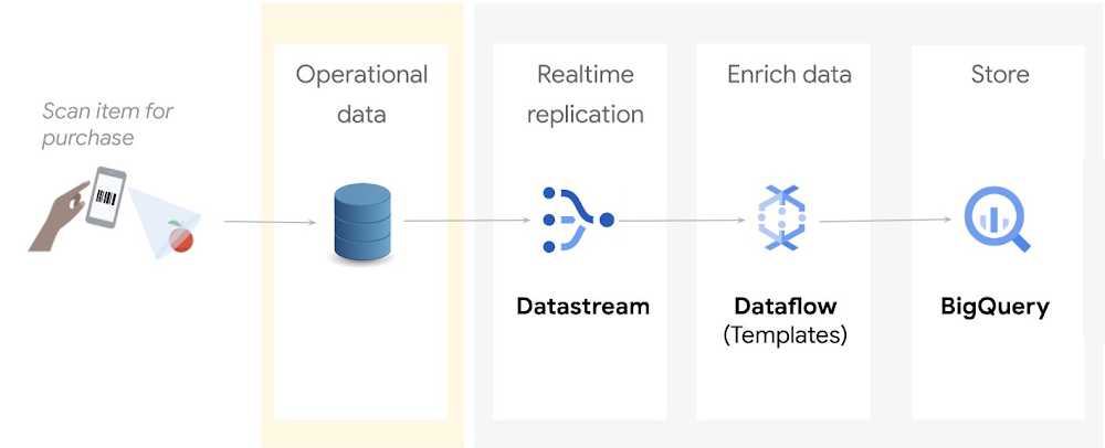
Relational databases are great at processing transactions, but they’re not designed to run analytics at scale. If you’re a data engineer or a data analyst, you may want to continuously replicate your operational data into a data warehouse in real time, so you can make timely, data driven business decisions.In this blog,  we will show you a step by step tutorial on how to replicate and process operational data from an Oracle database into Google Cloud’s BigQuery so that you can keep multiple systems in sync – minus the need for bulk load updating and inconvenient batch windows.The operational flow shown in the preceding diagram is as follows:Incoming data from an Oracle source is captured and replicated into Cloud Storage through Datastream.This data is processed and enriched by Dataflow templates, and is then sent to BigQuery for analytics and visualizationGoogle does not provide licenses for Oracle workloads. You are responsible for procuring licenses for the Oracle workloads that you choose to run on Google Cloud, and you are responsible for complying with the terms of these licenses. CostsThis tutorial uses the following billable components of Google Cloud:DatastreamCloud StoragePub/SubDataflowBigQueryCompute EngineTo generate a cost estimate based on your projected usage, use the pricing calculator.When you finish this tutorial, you can avoid continued billing by deleting the resources you created. For more information, see Clean up.Before you begin1. In the Google Cloud Console, on the project selector page, select or create a Google Cloud project.Note: If you don’t plan to keep the resources that you create in this procedure, create a project instead of selecting an existing project. After you finish these steps, you can delete the project, removing all resources associated with the project.2. Make sure that billing is enabled for your Cloud project. Learn how to check if billing is enabled on a project.3. Enable the Compute Engine, Datastream, Dataflow, and Pub/Sub APIs. 4. You must also have the role of Project owner or Editor.Step 1: Prepare your environment1. In Cloud Shell, define the following environment variables:code_block[StructValue([(u’code’, u’export PROJECT_NAME=”YOUR_PROJECT_NAME”rnexport PROJECT_ID=”YOUR_PROJECT_ID”rnexport PROJECT_NUMBER=”YOUR_PROJECT_NUMBER”rnexport BUCKET_NAME=”${PROJECT_ID}-oracle_retail”‘), (u’language’, u”)])]Replace the following:YOUR_PROJECT_NAME: The name of your projectYOUR_PROJECT_ID: The ID of your projectYOUR_PROJECT_NUMBER: The number of your project2. Enter the following:code_block[StructValue([(u’code’, u’gcloud config set project ${PROJECT_ID}’), (u’language’, u”)])]3. Clone the GitHub tutorial repository which contains the scripts and utilities that you use in this tutorial:code_block[StructValue([(u’code’, u’git clone \rnhttps://github.com/caugusto/datastream-bqml-looker-tutorial.git’), (u’language’, u”)])]4. Extract the comma-delimited file containing sample transactions to be loaded into Oracle:code_block[StructValue([(u’code’, u’bunzip2 \rndatastream-bqml-looker-tutorial/sample_data/oracle_data.csv.bz2′), (u’language’, u”)])]5. Create a sample Oracle XE 11g docker instance on Compute Engine by doing the following:a. In Cloud Shell, change the directory to build_docker:code_block[StructValue([(u’code’, u’cd datastream-bqml-looker-tutorial/build_docker’), (u’language’, u”)])]b. Run the following build_orcl.sh script:code_block[StructValue([(u’code’, u’./build_orcl.sh \rn-p <YOUR_PROJECT_ID> \rn-z <GCP_ZONE> \rn-n <GCP_NETWORK_NAME> \rn-s <GCP_SUBNET_NAME> \rn-f Y \rn-d Y’), (u’language’, u”)])]Replace the following:YOUR_PROJECT_ID: Your Cloud project IDGCP_ZONE: The zone where the compute instance will be createdGCP_NETWORK_NAME= The network name where VM and firewall entries will be createdGCP_SUBNET_NAME= The network subnet where VM and firewall entries will be createdY or N= A choice to create the FastFresh schema and ORDERS table (Y or N). Use Y for this tutorial.Y or N= A choice to configure the Oracle database for Datastream usage (Y or N). Use Y for this tutorial.The script does the following:Creates a new Google Cloud Compute instance.Configures an Oracle 11g XE docker container.Pre-loads the FastFresh schema and the Datastream prerequisites.After the script executes, the build_orcl.sh script gives you a summary of the connection details and credentials (DB Host, DB Port, and SID). Make a copy of these details because you use them later in this tutorial.After the script executes, the build_orcl.sh script gives you a summary of the connection details and credentials (DB Host, DB Port, and SID). Make a copy of these details because you use them later in this tutorial. 6. Create a Cloud Storage bucket to store your replicated data:code_block[StructValue([(u’code’, u’gsutil mb gs://${BUCKET_NAME}’), (u’language’, u”)])]Make a copy of the bucket name because you use it in a later step.7. Configure your bucket to send notifications about object changes to a Pub/Sub topic. This configuration is required by the Dataflow template. Do the following:a. Create a new topic called oracle_retail:code_block[StructValue([(u’code’, u’gsutil notification create -t projects/${PROJECT_ID}/topics/oracle_retail -f \rnjson gs://${BUCKET_NAME}’), (u’language’, u”)])]b. Create a Pub/Sub subscription to receive messages which are sent to the oracle_retail topic:code_block[StructValue([(u’code’, u’gcloud pubsub subscriptions create oracle_retail_sub \rn–topic=projects/${PROJECT_ID}/topics/oracle_retail’), (u’language’, u”)])]8. Create a BigQuery dataset named retail:code_block[StructValue([(u’code’, u’bq mk –dataset ${PROJECT_ID}:retail’), (u’language’, u”)])]9. Assign the BigQuery Admin role to your Compute Engine service account:code_block[StructValue([(u’code’, u”gcloud projects add-iam-policy-binding ${PROJECT_ID} \rn–member=serviceAccount:${PROJECT_NUMBER}-compute@developer.gserviceaccount.com \rn–role=’roles/bigquery.admin'”), (u’language’, u”)])]Step 2: Replicate Oracle data to Google Cloud with DatastreamDatastream supports the synchronization of data to Google Cloud databases and storage solutions from sources such as MySQL and Oracle.In this section, you use Datastream to backfill the Oracle FastFresh schema and to replicate updates from the Oracle database to Cloud Storage in real time.Create a stream1. In Cloud Console, navigate to Datastream and click Create Stream. A form appears. Fill in the form as follows, and then click Continue:Stream name: oracle-cdcStream ID: oracle-cdcSource type: OracleDestination type: Cloud StorageAll other fields: Retain the default value2. In the Define & Test Sourcesection, select Create new connection profile. A form appears. Fill in the form as follows, and then click Continue:Connection profile name: orcl-retail-sourceConnection profile ID: orcl-retail-sourceHostname: <db_host>Port: 1521Username: datastreamPassword: tutorial_datastreamSystem Identifier (SID): XEConnectivity method: Select IP allowlisting3. Click Run Test to verify that the source database and Datastream can communicate with each other, and then click Create & Continue.You see the Select Objects to Include page, which defines the objects to replicate, specific schemas, tables, and columns and be included or excluded.If the test fails, make the necessary changes to the form parameters and then retest.4. Select the following: FastFresh > Orders, as shown in the following image:5. To load existing records, set the Backfill mode to Automatic, and then click Continue. 6. In the Define Destination section, select Create new connection profile. A form appears. Fill in the form as follows, and then click Create & Continue:Connection Profile Name: oracle-retail-gcsConnection Profile ID: oracle-retail-gcsBucket Name: The name of the bucket that you created in the Prepare your environment section.7. Keep the Stream path prefix blank, and for Output format, select JSON. Click Continue.8. On the Create new connection profile page, click Run Validation, and then click Create.The output is similar to the following:Step 3: Create a Dataflow job using the Datastream to BigQuery templateIn this section, you deploy Dataflow’s Datastream to BigQuery streaming template to replicate the changes captured by Datastream into BigQuery.You also extend the functionality of this template by creating and using UDFs.Create a UDF for processing incoming dataYou create a UDF to perform the following operations on both the backfilled data and all new incoming data:Redact sensitive information such as the customer payment method.Add the Oracle source table to BigQuery for data lineage and discovery purposes.This logic is captured in a JavaScript file that takes the JSON files generated by Datastream as an input parameter.1. In the Cloud Shell session, copy and save the following code to a file named retail_transform.js:code_block[StructValue([(u’code’, u’function process(inJson) {rnrn var obj = JSON.parse(inJson),rn includePubsubMessage = obj.data && obj.attributes,rn data = includePubsubMessage ? obj.data : obj;rnrn data.PAYMENT_METHOD = data.PAYMENT_METHOD.split(‘:’)[0].concat(“XXX”);rnrn data.ORACLE_SOURCE = data._metadata_schema.concat(‘.’, data._metadata_table);rnrn return JSON.stringify(obj);rn}’), (u’language’, u”)])]2. Create a Cloud Storage bucket to store the retail_transform.js file and then upload the JavaScript file to the newly created bucket:code_block[StructValue([(u’code’, u’gsutil mb gs://js-${BUCKET_NAME}rnrngsutil cp retail_transform.js \rngs://js-${BUCKET_NAME}/utils/retail_transform.js’), (u’language’, u”)])]Create a Dataflow job1. In Cloud Shell, create a dead-letter queue (DLQ) bucket to be used by Dataflow:code_block[StructValue([(u’code’, u’gsutil mb gs://dlq-${BUCKET_NAME}’), (u’language’, u”)])]2. Create a service account for the Dataflow execution and assign the account the following roles: Dataflow Worker, Dataflow Admin, Pub/Sub Admin, BigQuery Data Editor,BigQuery Job User, Datastream Admin and Storage Admin.code_block[StructValue([(u’code’, u’gcloud iam service-accounts create df-tutorial’), (u’language’, u”)])]code_block[StructValue([(u’code’, u’gcloud projects add-iam-policy-binding ${PROJECT_ID} \rn–member=”serviceAccount:df-tutorial@${PROJECT_ID}.iam.gserviceaccount.com” \rn–role=”roles/dataflow.admin”rnrngcloud projects add-iam-policy-binding ${PROJECT_ID} \rn–member=”serviceAccount:df-tutorial@${PROJECT_ID}.iam.gserviceaccount.com” \rn–role=”roles/dataflow.worker”rnrngcloud projects add-iam-policy-binding ${PROJECT_ID} \rn–member=”serviceAccount:df-tutorial@${PROJECT_ID}.iam.gserviceaccount.com” \rn–role=”roles/pubsub.admin”rnrngcloud projects add-iam-policy-binding ${PROJECT_ID} \rn–member=”serviceAccount:df-tutorial@${PROJECT_ID}.iam.gserviceaccount.com” \rn–role=”roles/bigquery.dataEditor”rnrngcloud projects add-iam-policy-binding ${PROJECT_ID} \rn–member=”serviceAccount:df-tutorial@${PROJECT_ID}.iam.gserviceaccount.com” \rn–role=”roles/bigquery.jobUser”rnrngcloud projects add-iam-policy-binding ${PROJECT_ID} \rn–member=”serviceAccount:df-tutorial@${PROJECT_ID}.iam.gserviceaccount.com” \rn–role=”roles/datastream.admin”rnrnrngcloud projects add-iam-policy-binding ${PROJECT_ID} \rn–member=”serviceAccount:df-tutorial@${PROJECT_ID}.iam.gserviceaccount.com” \rn–role=”roles/storage.admin”‘), (u’language’, u”)])]3. Create a firewall egress rule to let Dataflow VMs communicate, send, and receive network traffic on TCP ports 12345 and 12346 when auto scaling is enabled:code_block[StructValue([(u’code’, u’gcloud compute firewall-rules create fw-allow-inter-dataflow-comm \rn–action=allow \rn–direction=ingress \rn–network=GCP_NETWORK_NAME \rn–target-tags=dataflow \rn–source-tags=dataflow \rn–priority=0 \rn–rules tcp:12345-12346′), (u’language’, u”)])]4. Create and run a Dataflow job:code_block[StructValue([(u’code’, u’export REGION=us-central1rnrngcloud dataflow flex-template run orders-cdc-template –region ${REGION} \rn–template-file-gcs-location “gs://dataflow-templates/latest/flex/Cloud_Datastream_to_BigQuery” \rn–service-account-email “df-tutorial@${PROJECT_ID}.iam.gserviceaccount.com” \rn–parameters \rninputFilePattern=”gs://${BUCKET_NAME}/”,\rngcsPubSubSubscription=”projects/${PROJECT_ID}/subscriptions/oracle_retail_sub”,\rninputFileFormat=”json”,\rnoutputStagingDatasetTemplate=”retail”,\rnoutputDatasetTemplate=”retail”,\rndeadLetterQueueDirectory=”gs://dlq-${BUCKET_NAME}”,\rnautoscalingAlgorithm=”THROUGHPUT_BASED”,\rnmergeFrequencyMinutes=1,\rnjavascriptTextTransformGcsPath=”gs://js-${BUCKET_NAME}/utils/retail_transform.js”,\rnjavascriptTextTransformFunctionName=”process”‘), (u’language’, u”)])]Check the Dataflow console to verify that a new streaming job has started.5. In Cloud Shell, run the following command to start your Datastream stream:code_block[StructValue([(u’code’, u’gcloud datastream streams update oracle-cdc \rn–location=us-central1 –state=RUNNING –update-mask=state’), (u’language’, u”)])]6. Check the Datastream stream status:code_block[StructValue([(u’code’, u’gcloud datastream streams list –location=us-central1′), (u’language’, u”)])]Validate that the state shows as Running. It may take a few seconds for the new state value to be reflected.Check the Datastream console to validate the progress of the ORDERS table backfill.The output is similar to the following:Because this task is an initial load, Datastream reads from the ORDERS object. It writes all records to the JSON files located in the Cloud Storage bucket that you specified during the stream creation. It will take about 10 minutes for the backfill task to complete.Final step: Analyze your data in BigQueryAfter a few minutes, your backfilled data replicates into BigQuery. Any new incoming data is streamed into your datasets in (near) real time. Each record is processed by the UDF logic that you defined as part of the Dataflow template.The following two new tables in the datasets are created by the Dataflow job:ORDERS: This output table is a replica of the Oracle table and includes the transformations applied to the data as part of the Dataflow template.ORDERS_log: This staging table records all the changes from your Oracle source. The table is partitioned, and stores the updated record alongside some metadata change information, such as whether the change is an update, insert, or delete.BigQuery lets you see a real-time view of the operational data. You can also run queries such as a comparison of the sales of a particular product across stores in real time, or combining sales and customer data to analyze the spending habits of customers in particular stores.Run queries against your operational data1. In BigQuery, run the following SQL to query the top three selling products:code_block[StructValue([(u’code’, u’SELECT product_name, SUM(quantity) as total_salesrnFROM `retail.ORDERS`rnGROUP BY product_namernORDER BY total_sales descrnLIMIT 3;’), (u’language’, u”)])]The output is similar to the following:2. In BigQuery, run the following SQL statements to query the number of rows on both the ORDERS and ORDERS_log tables:code_block[StructValue([(u’code’, u’SELECT count(*) FROM `hackfast.retail.ORDERS_log`;rnSELECT count(*) FROM `hackfast.retail.ORDERS`;’), (u’language’, u”)])]With the backfill completed, the last statement should return the number 520217.Congratulations! Now you just completed the change data capture of Oracle data in BigQuery, real-time!Clean upTo avoid incurring charges to your Google Cloud account for the resources used in this tutorial, either delete the project that contains the resources, or keep the project and delete the individual resources. To remove the project:In the Cloud console, go to the Manage resources page.In the project list, select the project that you want to delete, and then click Delete.In the dialog, type the project ID, and then click Shut down to delete the project.What’s next?If you’re looking to further build on this foundation, wonder how to forecast future demand, and how to visualize this forecast data as it arrives, explore this tutorial: Build and visualize demand forecast predictions using Datastream, Dataflow, BigQuery ML, and Looker.Related ArticleSecurely exchange data and analytics assets at scale with Analytics Hub, now available in previewEfficiently and securely exchange valuable data and analytics assets across organizational boundaries with Analytics Hub. Start your free…Read Article
Quelle: Google Cloud Platform

GKE workload rightsizing — from recommendations to action

Do you know how to rightsize a workload in Kubernetes? If you’re not 100% sure, we have some great news for you! Today, we are launching a fully embedded, out-of-the-box experience to help you with that complex task. When you run your applications on Google Kubernetes Engine (GKE), you now get an end-to-end workflow that helps you discover optimization opportunities, understand workload specific resource request suggestions and, most importantly, act on those recommendations — all in a matter of seconds.This workload optimization workflow helps rightsize applications by looking at Kubernetes resource requests and limits, which are often one of the largest sources of resource waste. Correctly configuring your resource requests can be the difference between an idle cluster and a cluster that has been downscaled in response to actual resource usage.If you’re new to GKE, you can save time and money by following the rightsizer’s recommended resource request settings. If you’re already running workloads on GKE, you can also use it to quickly assess optimization opportunities for your existing deployments.Then, to optimize your workloads even more, combine these new workload rightsizing capabilities with GKE Autopilot, which is priced based on Pod resource requests. With GKE Autopilot, any optimizations you make to your Pod resource requests (assuming they are over the minimum) are directly reflected on your bill.We’re also introducing a new metric for Cloud Monitoring that provides resource requests suggestions for each individual eligible workload, based on its actual usage over time.Seamless workload rightsizing with GKEWhen you run a workload on GKE, you can use cost optimization insights to discover your cluster and workload rightsizing opportunities right in the console.Here, you can see your workload’s actual usage and get signals for potentially undersized workloads that are at risk of either reliability or performance impact because they have low resource requests.However, taking the next step and correctly rightsizing those applications has always been a challenge — especially at scale. Not anymore with GKE’s new workload rightsizing capability.Start by picking up the workload you want to optimize. Usually, the best candidates are the ones where there’s a considerable divergence between resource requests and limits and actual usage. In the cost optimization tab of the GKE workloads console, just look for the workloads with a lot of bright green.Once you pick a workload, go to workload details and choose “Actions” => “Scale” => “Edit resource requests” to get more step-by-step optimization guidance.The guidance you receive relies heavily on new “Recommended per replica request cores” and “Recommended per replica request bytes” metrics (the same metrics that are available in Cloud Monitoring), which are both based on actual workload usage. You can access this view for every eligible GKE deployment, with no configuration on your part.Once you confirm the values that are best for your deployment, you can edit the resource requests and limits directly in the GKE console, and they will be directly applied to your workloads.Note: Suggestions are based on the observed usage patterns of your workloads and might not always be the best fit for your application. Each case might have its corner cases and specific needs. We advise a comprehensive check and understanding of values that are best for your specific workload.Note: Due to limited visibility into the way Java workloads use memory, we do not support memory recommendations for JVM-based workloads.Optionally, if you’d rather set the resource requests and limits from outside the GKE console, you can generate a YAML file with the recommended settings that you can use to configure your deployments.Note: Workloads with horizontal pod autoscaling enabled will not receive suggested values on the same metric for which horizontal pod autoscaling is configured. For instance, if your workload has HPA configured for CPU, only memory suggestions will be displayed.For more information about specific workload eligibility and compatibility with other scaling mechanisms such as horizontal pod autoscaling, check out the feature documentation here.Next-level efficiency with GKE Autopilot and workload rightsizingWe’ve talked extensively about GKE Autopilot as one of GKE’s key cost optimization mechanisms. GKE Autopilot provides a fully managed infrastructure offering that eliminates the need for nodepool and VM-level optimization, thus removing the bin-packing optimization challenges related to operating VMs, as well as unnecessary resource waste and day-two operations efforts. In GKE Autopilot, you pay for the resources you request. Combined with workload rightsizing, which primarily targets resource request optimization, you can easily now address two out of three main issues that lead to optimization gaps: app right-sizing and bin-packing. By running eligible workloads on GKE Autopilot and improving their resource requests, you should start to see a direct, positive impact on your bill right away!Rightsizing metrics and more resources for optimizing GKETo support the new optimization workflow we also launched two new metrics called “Recommended per replica request cores” and “Recommended per replica request bytes”. Both are available in the Kubernetes Scale metric group in Cloud Monitoring under “Kubernetes Scale” => “Autoscaler” => “Recommended per replica request”. You can also use these metrics to  build your own customization and ranking views and experiences, and export latest optimization opportunities.Excited about the new optimization opportunities? Ready for a recap of many other things you could do to run GKE more optimally? Check our Best Practices for Running Cost Effective Kubernetes Applications, the Youtube series, and have a look at the GKE best practices to lessen overprovisioning.Related ArticleGoogle Cloud at KubeCon EU: New projects, updated services, and how to connectEngage with experts and learn more about Google Kubernetes Engine at KubeCon EU.Read Article
Quelle: Google Cloud Platform

Announcing PSP's cryptographic hardware offload at scale is now open source

Almost a decade ago, we started encrypting traffic between our data centers to help protect user privacy. Since then, we gradually rolled out changes to encrypt almost all data in transit. Our approach is described in our Encryption in Transit whitepaper. While this effort provided invaluable privacy and security benefits, software encryption came at significant cost: it took ~0.7% of Google’s processing power to encrypt and decrypt RPCs, along with a corresponding amount of memory. Such costs spurred us to offload encryption to our network interface cards (NICs) using PSP (a recursive acronym for PSP Security Protocol), which we are open sourcing today.Google’s production machines are shared among multiple tenants that have strict isolation requirements. Hence, we require per-connection encryption and authentication, similar to Transport Layer Security (TLS). At Google’s scale, the implication is that the cryptographic offload must support millions of live Transmission Control Protocol (TCP) connections and sustain 100,000 new connections per second at peak. Before inventing a new offload-friendly protocol, we investigated existing industry-standards: Transport Layer Security (TLS) and Internet Protocol Security (IPsec). While TLS meets our security requirements, it is not an-offload friendly solution because of the tight coupling between the connection state in the kernel and the offload state in hardware. TLS also does not support non-TCP transport protocols, such as UDP. IPsec protocol, on the other hand, is transport independent and can be offloaded to hardware. However, a limitation of IPSec offload solutions is that they cannot economically support our scale partly because they store the full encryption state in an associative hardware table with modest update rates. Assuming the size of an entry is 256B in either direction, transmit or receive, the total memory requirement for 10M connections is 5GB (256B x 2 x 10M) – which is well beyond the affordable capacity of commodity offload engines. Existing IPsec offload engines are designed to support encryption for a small number of site-to-site tunnels. Ultimately, we decided that IPsec does not meet our security requirements as it lacks support for keys per layer-4 connection.To address these challenges, we developed PSP (a recursive acronym for PSP Security Protocol,) a TLS-like protocol that is transport-independent, enables per-connection security, and is offload-friendly.At Google, we employ all of these protocols depending on the use case. For example, we use TLS for our user-facing connections, we use IPsec for site-to-site encryption where we need interoperability with 3rd party appliances, and we use PSP for intra- and inter- data center traffic.PSP is intentionally designed to meet the requirements of large-scale data-center traffic. It does not mandate a specific key exchange protocol and offers few choices for the packet format and the cryptographic algorithms. It enables per-connection security by allowing an encryption key per layer-4 connection (such as a TCP connection.) It supports stateless operation because the encryption state can be passed to the device in the packet descriptor when transmitting packets and can be derived when receiving packets using a Security Parameter Index (SPI) and an on-device master key. This enables us to maintain minimal state in the hardware, avoiding hardware state explosion compared to typical stateful encryption technologies maintaining large on-device tables.PSP supports both stateful and stateless modes of operation: In the stateless mode, encryption keys are stored in the transmit packet descriptors and derived for received packets, using a master key stored on the device. In contrast, stateful technologies typically maintain the actual encryption keys in a table per connection.PSP uses User Datagram Protocol (UDP) encapsulation with a custom header and trailer. A PSP packet starts with the original IP header, followed by a UDP header on a prespecified destination port, followed by a PSP header containing the PSP information, followed by the original TCP/UDP packet (including header and payload), and ends with a PSP trailer that contains an Integrity Checksum Value (ICV). The layer-4 packet (header and payload) can be encrypted or authenticated, based on a user-provided offset called Crypt Offset. This field can be used to, for example, leave part of the TCP header authenticated yet unencrypted in transit while keeping the rest of the packet encrypted to support packet sampling and inspection in the network if necessary.  This is a critical visibility feature for us enabling proper attribution of traffic to applications, and is not feasible to achieve with IPsec. Of note, the UDP header is protected by the UDP checksum and the PSP header is always authenticated.PSP packet format for encrypting a simple TCP/IP packet in the Linux TCP/IP stack.We support PSP in our production Linux kernel, Andromeda (our network virtualization stack), and Snap (our host networking system), enabling us to use PSP for both internal communication and for Cloud customers. As of 2022, PSP cryptographic offload saves 0.5% of Google’s processing power. Similar to any other cryptographic protocol, we need both ends of a connection to support PSP. This can be prohibitive in brownfield deployments with a mix of old and new (PSP-capable) NICs. We built a software implementation of PSP (SoftPSP) to allow PSP-capable NICs to communicate with older machines, dramatically increasing coverage among pairwise server connections.PSP delivers multiplicative benefits when combined with zero-copy techniques. For example, the impact of TCP zero-copy for both sending and receiving was limited by extra reads and writes of the payloads for software encryption. Since PSP eliminates these extra loads and stores, RPC processing no longer requires touching the payload in the network stack. For large 1MB RPCs, for example, we see a 3x speed up from combining PSP and zero-copy.PSP and ZeroCopy have multiplicative impact, enabling us to send and receive RPCs without touching the payload. For large 1MB RPCs, using PSP alongside Zero-copy increases the throughput of TCP channels by 3x.We believe that PSP can provide a number of significant security benefits for the industry. Given its proven track record in our production environment, we hope that it can become a standard for scalable, secure communication across a wide range of settings and applications. To support this, we are making PSP open source to encourage broader adoption by the community and hardware implementation by additional NIC vendors. For further information, please refer to http://github.com/google/psp which includes:The PSP Architecture Specification.A reference software implementation.A suite of test cases.For further questions and discussions, please join the PSP discussion Google Group or contact the group here: psp-discuss@googlegroups.com.Acknowledgements: We are thankful to a large number of colleagues from Technical Infrastructure and Cloud who contributed to PSP since its inception, including but not limited to Platforms, Security, Kernel Networking, RPCs, Andromeda, and other Network Infrastructure teams.Related ArticleIntroducing Google Cloud’s new Assured Open Source Software serviceAnnouncing Google Cloud’s new Assured Open Source Software Service, which can help organizations add the same software that Google uses i…Read Article
Quelle: Google Cloud Platform

New Research shows Google Cloud Skill Badges build in-demand expertise

We live in a digital world, and the future of work is in the cloud. In fact, 61% of HR professionals believe hiring developers will be their biggest challenge in the years ahead.1During your personal cloud journey, it’s critical to build and validate your skills in order to evolve with the rapidly changing technology and business landscape.That is why we created skill badges – a micro-credential issued by Google Cloud to demonstrate your cloud competencies and your commitment to staying on top of the latest Google Cloud solutions and products. To better understand the value of skills badges to holders’ career goals, we commissioned a third-party research firm, Gallup, to conduct a global study on the impact of Google Cloud skill badges. Skill badge earners overwhelmingly gain value from and are satisfied with Google Cloud skill badges.Skill badge holders state that they feel well equipped with the variety of skills gained through skill badge attainment, that they are more confident in their cloud skills, are excited to promote their skills to their professional network, and are able to leverage skill badges to achieve future learning goals, including a Google Cloud certification. 87% agree skill badges provided real-world, hands-on cloud experience286% agree skill badges helped build their cloud competencies2 82% agree skill badges helped showcase growing cloud skills290% agree that skill badges helped them in their Google Cloud certification journey274% plan to complete a Google Cloud certification in the next six months2Join thousands of other learners and take your career to the next level with Google Cloud skill badges.To learn more, download the Google Cloud Skills Badge Impact Report at no cost.1. McKinsey Digital,Tech Talent Technotics: Ten new realities for finding, keeping, and developing talent , 20222. Gallup Study, sponsored by Google Cloud Learning: “Google Cloud Skill Badge Impact report”, May 2022Related ArticleHow to prepare for — and ace — Google’s Associate Cloud Engineer examThe Cloud Engineer Learning Path is an effective way to prepare for the Associate.Read Article
Quelle: Google Cloud Platform

AWS Distribution of Kubeflow, mit Support für Kubeflow v1.4.1, ist jetzt allgemein verfügbar

Wir freuen uns, heute die allgemeine Verfügbarkeit des AWS-Supports für Kubeflow v1.4 bekannt geben zu können. Kubeflow in AWS rationalisiert die Aufgaben der Datenwissenschaft und hilft beim Entwickeln äußerst zuverlässiger, sicherer, portabler und skalierbarer ML-Systeme mit reduzierten Betriebskosten durch die Integration mit AWS Managed Services. Mit dieser Kubeflow-Verteilung können Sie ML-Systeme auf der Grundlage von Amazon Elastic Kubernetes Service (Amazon EKS) entwickeln, trainieren und optimieren und ML-Modelle für eine Vielzahl von Anwendungsfällen bereitstellen. Darunter sind auch Computer Vision, die natürliche Sprachverarbeitung, die Sprachübersetzung und die Finanzmodellierung.
Quelle: aws.amazon.com

AWS Control Tower kann jetzt vom Kunden bereitgestellte Kernkonten verwenden

Heute kündigen wir eine neue Funktion in AWS Control Tower an, die Ihnen die Flexibilität bietet, Ihre bestehenden Sicherheits- und Protokollierungskonten zu verwenden. Außerdem können Sie bei der Einrichtung von Control Tower und bei der Erweiterung der Governance auf bestehende AWS-Umgebungen neue Konten in Ihrem Namen erstellen. Das Sicherheitskonto wird als eingeschränktes Konto verwendet, mit dem Ihre Sicherheits- und Compliance-Teams Lese- und Schreibzugriff auf alle Konten in Ihrer Landing Zone erhalten. Das Protokollierungskonto dient als Repository, in dem Protokolle von API-Aktivitäten und Ressourcenkonfigurationen aller Konten in Ihrer Landing Zone gespeichert werden. 
Quelle: aws.amazon.com

Amazon Lex unterstützt nun auch Ausdruckshinweise

Amazon Lex bietet Funktionen zur automatischen Spracherkennung und zum Verstehen natürlicher Sprache, sodass Sie Anwendungen und interaktive Sprachdialoglösungen mit ansprechenden Benutzererlebnissen erstellen können. Ab heute können Sie während einer Live-Interaktion programmgesteuert Ausdrücke als Hinweise bereitstellen, um die Transkription der gesprochenen Eingabe zu beeinflussen. Bei der Interaktion mit der Sprachdialoglösung einer Bank könnte ein Kunde beispielsweise einen Spitznamen („Smythes Girokonto“) für das Zielkonto verwenden. Sie können Geschäftslogik ausführen, um alle Spitznamen von Zahlungsempfängern zu identifizieren, die mit dem Konto des Anrufers verbunden sind, und diese als Hinweise bereitstellen, um die Transkription von Namen zu verbessern. Eine bessere Erkennung führt zu effizienteren Konversationen und erhöht letztlich die Kundenzufriedenheit.
Quelle: aws.amazon.com

X2idn- und X2iedn-Instances von Amazon EC2 sind jetzt in 8 zusätzlichen Regionen verfügbar

Ab heute sind arbeitsspeicheroptimierte X2idn- und X2iedn-Instances von Amazon EC2 in folgenden zusätzlichen Regionen verfügbar: Asien-Pazifik (Seoul, Sydney), Kanada (Zentral), Europa (London, Stockholm, Mailand), Südamerika (São Paulo) und AWS GovCloud (USA-Ost). X2idn- und X2iedn-Instances wurden für speicherintensive Workloads entwickelt und bieten im Vergleich zu den X1-Instances der vorherigen Generation verbesserte Leistung, Preis und Kosten pro GiB Speicher. Diese neuen Instances werden von skalierbaren Intel-Xeon-Prozessoren der 3. Generation (Ice Lake) angetrieben und bieten ein bis zu 50 % verbessertes Computing-Preisleistungverhältnis im vergleich zu X1-Instances. Bei X2idn ist das Verhältnis von Speicher zu vCPU gleich 16:1, und bei X2iedn gleich 32:1, wodurch sich diese Instances hervorragend für Workloads wie In-Memory-Datenbanken und -Analysen, Big-Data-Verarbeitungsmaschinen und EDA-Workloads (Electronic Design Automation) eignen.
Quelle: aws.amazon.com