Adventures: Kreuzfahrt in den Tod und andere Abenteuer
Gattenmord auf dem Traumschiff in Overboard und Bären als Mafiosi in Backbone: Golem.de stellt die besten neuen Adventures vor. Von Rainer Sigl (Adventure, Spieletest)
Quelle: Golem

Gattenmord auf dem Traumschiff in Overboard und Bären als Mafiosi in Backbone: Golem.de stellt die besten neuen Adventures vor. Von Rainer Sigl (Adventure, Spieletest)
Quelle: Golem

Steven Spielbergs Produktionsfirma wird pro Jahr mehrere Spielfilme exklusiv für Netflix produzieren. (Netflix, Streaming)
Quelle: Golem

Apple soll ein Macbook Air mit einem flacheren Gehäuse, einem neuen Prozessor und in vielen verschiedenen Farben planen. (Macbook Air, Apple)
Quelle: Golem

Das Rokit enthält ein Qualcomm-SoC, entsperrtes Android und ein biegsames Amoled-Display für Bastelideen. Das alles wird im Koffer verstaut. (OLED, Mobil)
Quelle: Golem

Ein EZB-Direktor positioniert den geplanten digitalen Euro als Alternative zu sogenannten Kryptowährungen. (E-Commerce, Datenschutz)
Quelle: Golem
As part of the Red Hat “Leap into RHEL 8 Giveaway,” we will give swag to the first 500 people to migrate a system to RHEL 8 through July 31.
The giveaways include a t-shirt and blue-light blocking glasses, which you can earn in two ways:
Quelle: CloudForms
Earlier this year, Red Hat Process Automation subscribers gained access to Kogito-based capabilities. This release was the first version of Red Hat Process Automation to introduce components of Kogito, an open source community project that seeks to create the next generation of business automation technology.
Quelle: CloudForms
The SSH server is a critical, ubiquitous service that provides one of the main access points into Red Hat Enterprise Linux (RHEL) for management purposes. Over my career as a system administrator, I can not think of any RHEL systems I have worked on that were not running it.
Quelle: CloudForms
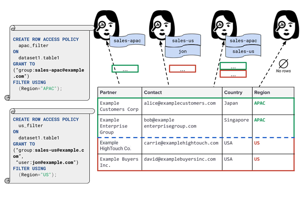
Data security is an ongoing concern for anyone managing a data warehouse. Organizations need to control access to data, down to the granular level, for secure access to data both internally and externally. With the complexity of data platforms increasing day by day, it’s become even more critical to identify and monitor access to sensitive data. In many cases, sensitive data is co-mingled with non-sensitive data, and access restrictions to sensitive data need to be enabled based on factors like data location or presence of financial information. There may also be nuances where data is sensitive for some groups of users, while for others, it is not. Today, we’re pleased to announce the general availability of BigQuery row-level security, which gives customers a way to control access to subsets of data in the same table for different groups of users. Row-level security (RLS) extends the principle of least privilege access and enables fine-grained access control policies in BigQuery tables. BigQuery currently supports access controls at the project-, dataset-, table- and column-level. Adding RLS to the portfolio of access controls now enables customers to filter and define access to specific rows in a table based on qualifying user conditions—providing much needed peace of mind for data professionals. “Our digital transformation and migration of data to the cloud magnifies the business value we can extract from our information assets. However, granular data access control is essential to comply with international regulatory and contractual requirements. BigQuery row-level security helps us comply with data residency and export restrictions,” says Jarrett Garcia, Iron Mountain’s Enterprise Data Platform Senior Director. “It enables us to manage fine-grained access controls without replicating data. What used to take months for approval and access provisioning can now be done more efficiently and effectively. We are looking forward to implementing additional data security capabilities on the BigQuery roadmap to address other critical business use cases.”How BigQuery row-level security worksRow-level security in BigQuery enables different user personas access to subsets of data in the same table. Customers who are currently using authorized views to enable these use cases can leverage RLS for ease of management. To express the concept of RLS, we have introduced a new entity in BigQuery called row access policy. Row access policies map a group of user principals to the rows that they can see, defined by a SQL filter predicate. Secure logic rules created by data owners and administrators determines which user can see which rows through the creation of a row-level access policy. The row-level access policies created on a target table by administrators or data owners are applied when a query is run on the table. One table can have multiple policies applied to it.Below is an example, where row-level access policies have been created to filter data based on users’ “region”.Click to enlargeIn the illustrated scenario above, row-level access policies have been created to verify a querying user’s region and to give them access only to the subset of data relevant to that region. Access policies are granted to a grantee list which support all types of IAM principles such as individual users, groups, domains or service accounts. In this example, when a user queries the table, row-level access policies are evaluated to assess which, if any, policies are applicable to that user. The group ‘sales-apac’ is granted access to view a subset of rows where region = ‘APAC’ whereas the group ‘sales-us’ is granted access to view a subset of rows where the region = ’US’. Likewise, users in both groups will see rows in both regions, and users in neither group will not see any rows.Row-level access policies can also be created using the SESSION_USER() function to restrict access only to rows that belong to the user running the query. If none of the row access policies are applicable to the querying user, the user will have no access to the data in the table.When a user queries a table with a row-level access policy, BigQuery displays a banner notice indicating that their results may be filtered by a row-level access policy. This notice displays even if the user is a member of the `grantee_list`.Click to enlargeWhen to put BigQuery row-level security to workRow-level access policies are useful when you have a need to limit access to data based on filter conditions. The row-access policies’ filter predicate supports arbitrary SQL, and is conceptually similar to the WHERE clause of a SQL query. Filter predicates support the SESSION_USER() function to restrict access only to rows that belong to the user running the query. If none of the row access policies are applicable to the querying user, the user will have no access to the data in the table. Currently, the column used for filtering must be in the table, but we anticipate adding support for subqueries in the filter expression, opening up access to use cases where data is filtered based on lookup tables and calculated values. Row-level access policies can be created, updated and dropped using DDL statements. You will be able to see the list of row-level access policies applied to a table using the BigQuery schema pane in the Cloud Console, which simplifies the management of policies per table, or by using the bq command-line tool.Click to enlargeRow-level security is compatible with other BigQuery security features, and can be used along with column-level security for further granularity. Since row-level access policies are applied on the source tables, any actions performed on the table will inherit the table’s associated access policies, to ensure access to secure data is protected. Row-level access policies are applicable to every method used to access BigQuery data (API, Views, etc). Try it outWe’re always working to enhance BigQuery’s (and Google Cloud’s) data governance capabilities, to provide more controls around managing your data. With row-level security, we are adding deeper protections for your data. You can learn more about BigQuery row-level security in our documentation and best practices.Related ArticleData governance in Google Cloud–new ways to securely access and discover dataAs organizations bring ever more sensitive data analytics workloads to the cloud, BigQuery column-level security, now GA, provides fine-g…Read Article
Quelle: Google Cloud Platform
Geospatial data is a critical component for a comprehensive analytics strategy. Whether you are trying to visualize data using geospatial parameters or do deeper analysis or modeling on customer distribution or proximity, most organizations have some type of geospatial data they would like to use – whether it be customer zipcodes, store locations, or shipping addresses. However, converting geographic data into the correct format for analysis and aggregation at different levels can be difficult. In this post, we’ll walk through some examples of how you can leverage the Google Cloud platform alongside Google Cloud Public Datasets to perform robust analytics on geographic data. The full queries can be accessed from this notebook here. Public US Geo Boundaries datasetBigQuery hosts a slew of public datasets for you to access and integrate into your analytics. Google pays for the storage of these datasets and provides public access to the data via the bigquery-public-data project. You only pay for queries against the data. Plus, the first 1 TB per month is free! These public datasets are valuable on their own, but when joined against your own data they can unlock new analytics use cases and save the team a lot of time. Within the Google Cloud Public Datasets Program there are several geographic datasets. Here, we’ll work with the geo_us_boundaries dataset, which contains a set of tables that have the boundaries of different geospatial areas as polygons and coordinates based on the center point (GEOGRAPHY column type in BigQuery), published by the US Census Bureau.Mapping geospatial points to hierarchical areasMany times you will find yourself in situations where you have a string representing an address. However, most tools require lat/long coordinates to actually plot points. Using theGoogle Maps Geocoding API we can convert an address into a lat/long and then store the results in the BigQuery table. With a lat/long representation of our point, we can join our initial dataset back onto any of the tables here using the ST_WITHIN function. This allows us to check and see if a point is within the specified polygon. ST_WITHIN(geography_1, geography_2)This can be helpful for ensuring standard nomenclature; for example, metropolitan areas that might be named differently. The query below maps each customers’ address to a given metropolitan area name.It can also be useful for converting to designated market area (DMA), which is often used in creating targeted digital marketing campaigns.Or for filling in missing information; for example, some addresses may be missing zip code which results in incorrect calculations when aggregating up to the zipcode level. By joining onto the zip_codes table we can ensure all coordinates are mapped appropriately and aggregate up from there.Note that the zip code table isn’t a comprehensive list of all US zip codes, they are zip code tabulation areas (ZCTAs). Details about the differences can be found here. Additionally, the zip code table gives us hierarchical information, which allows us to perform more meaningful analytics. One example is leveraging hierarchical drilling in Looker. I can aggregate my total sales up to the country level, and then drill down to state, city and zipcode to identify where sales are highest. You can also use the BigQuery GeoViz tool to visualize geospatial data!Aside from simply checking if a point is within an area, we can also use ST_DISTANCE to do something like find the closest city using the centerpoint for the metropolitan area table. This concept doesn’t just hold true for points, we can also leverage other GIS functions to see if a geospatial area is contained within areas that are listed in the boundaries datasets. If your data comes into BigQuery as a GeoJSON string, we can convert it to a GEOGRAPHY type using the ST_GEOGFROMGEOJSON function. Once our data is in a GEOGRAPHY type we can do things like check to see what urban area the geo is within – using either ST_WITHIN or ST_INTERSECTS to account for partial coverage. Here, I am using the customer’s zip code to find all metropolitan divisions where the zip code polygon and the metropolitan polygon intersect. I am then selecting the metropolitan area that has the most overlap (or the intersection has the largest area) to be the customer’s metro that we use for reporting.The same ideas can be applied to the other tables in the dataset including the county, urban areas and National Weather Service forecast regions (which can also be useful if you want to join your datasets onto weather data).Correcting for data discrepancyOne problem that we may run into when working with geospatial data is that different data sources may have different representations of the same information. For example, you might have one system that records state as a two letter abbreviation and another using the full name. Here, we can use the state table to join the different datasets.Another example might be using the tables as a source of truth for fuzzy matching. If the address is a manually entered field somewhere in your application, there is a good chance that things will be misspelled. Different representations of the same name may prevent tables from joining with each other or lead to duplicate entries when performing aggregations. Here, I use a simple Soundex algorithm to generate a code for each county name, using helper functions fromthis blog post. We can see that even though some are misspelled they have the same Soundex code.Next, we can join back onto our counties table so we make sure to use the correct spelling of the county name. Then, we can simply aggregate our data for more accurate reporting. Note that fuzzy matching definitely isn’t perfect and you might need to try different methods or apply certain filters for it to work best depending on the specifics of your data.The US Geo Boundary datasets allow you to perform meaningful geographic analysis without needing to worry about extracting, transforming or loading additional datasets into BigQuery. These datasets, along with all the other Google Cloud Public Datasets, will be available in the Analytics Hub. Please sign up for the Analytics Hub preview, which is scheduled to be available in the third quarter of 2021, by going to g.co/cloud/analytics-hub.Related ArticleIntroducing Analytics Hub: secure and scalable sharing for data and analyticsAnalytics Hub makes data sharing across organizations secure and easyRead Article
Quelle: Google Cloud Platform