Mirantis to take over support of Kubernetes dockershim

The post Mirantis to take over support of Kubernetes dockershim appeared first on Mirantis | Pure Play Open Cloud.
The rumors of dockershim’s demise have been greatly exaggerated. If you follow the Kubernetes ecosystem, you may have been caught up in the consternation excitement over the announcement that starting with the soon-to-be-released Kubernetes 1.20, users will receive a warning that dockershim is being deprecated, and will be removed in a future release. For many people this has sparked a moment of panic, but take a deep breath, everything is going to be OK.
Even better news, however, is that Mirantis and Docker have agreed to partner to maintain the shim code standalone outside Kubernetes, as a conformant CRI interface for the Docker Engine API. For Mirantis customers, that means that Docker Engine’s commercially supported version, Mirantis Container Runtime (MCR), will be CRI compliant. We will start with the great initial prototype from Dims at https://github.com/dims/cri-dockerd and continue to make it available as an open source project, https://github.com/Mirantis/cri-dockerd. This means that you can continue to build Kubernetes based on the Docker Engine as before, just switching from the built in dockershim to the external one. We will work together on making sure it continues to work as well as before and that it passes all the conformance tests and continues to work just like the built in version did. Mirantis will be using this in Mirantis Kubernetes Engine, and Docker will continue to ship this shim in Docker Desktop.
In the beginning…
If you work with Kubernetes, you know that it orchestrates containers. For many people, “container” means “Docker”, but that’s not strictly true. Docker revolutionized containers and brought them into common usage, and as such, the Docker Engine was the first (and originally the only) container runtime to be supported by Kubernetes.
But that was never the Kubernetes community’s long term plan.
Long term, the community wanted the ability to run many different types of containers (remember rkt?) and as such, created the Container Runtime Interface (CRI), a standard way for container engines to communicate with Kubernetes. If a container engine is CRI compliant, it can run in Kubernetes with no extra effort.
The first CRI-compliant container engine was containerd, which was derived from the guts of … wait for it… Docker. You see, Docker is more than just a container runtime; it includes other pieces that are meant for human consumption, such as the user interface. So Docker pulled out the pieces that were actually relevant as containerd, and it became the first CRI-compliant runtime. It then donated containerd to the Cloud Native Computing Foundation (CNCF). The cri-containerd component is runtime agnostic and supports multiple Linux operations systems, as well as Windows.
However, that left one problem. Docker itself still wasn’t CRI-compliant.
What is dockershim?
Just as Kubernetes started out with built-in support for Docker Engine, it also included built-in support for various storage volume solutions, network solutions, and even cloud providers. But maintaining these things on an ongoing basis became too cumbersome, so the community decided to strip all third party solutions out of the core, creating the relevant interfaces, such as:

Container Runtime Interface (CRI)
Container Network Interface (CNI)
Container Storage Interface (CSI)

The idea was that any vendor could create a product that automatically interfaces with Kubernetes, as long as it is compliant with these interfaces.
That doesn’t mean that non-compliant components can’t be used with Kubernetes; Kubernetes can do anything with the right components. It just means that non-compliant components need a “shim”, which translates between the component and the relevant Kubernetes interface. For example, dockershim takes CRI commands and translates them into something Docker Engine understands, and vice versa. But with the drive to take third-party components like this out of the Kubernetes core, dockershim had to be removed.
As dramatic as this sounds, however, it’s less of an issue than you think; the images you build with docker build are compliant with the underlying standard CRI uses, so they are still going to work with Kubernetes.
What happens now that built in dockershim support is deprecated in Kubernetes?
For most people, the deprecation of dockershim is a non-issue, because even though they’re not aware of it, they’re not actually using Docker per se; they’re using containerd, which is CRI compliant. For those people nothing will change.
Some people, however, including many Mirantis customers, are running workloads that are dependent on dockershim in order to work seamlessly with Kubernetes.
Because it’s still a necessary real-world component for many companies, Mirantis and Docker have agreed to continue supporting and developing dockershim, and to continue its status as a standalone open source component.
So what does this mean in actuality?
If you’re using containerd directly, you don’t have to worry about this at all; containerd will work with the CRI. If you’re a Mirantis customer, you also won’t have to worry about this; dockershim support will be included with the Mirantis Container Runtime, making it CRI-compliant.
Otherwise, if you’re using the open source Docker Engine, the dockershim project will be available as an open source component, and you will be able to continue to use it with Kubernetes; it will just require a small configuration change, which we will document.
So even though this came as a shock to many people, nobody is being left out in the cold.
If you’re looking for more information, the community has put out an FAQ and blog post giving more detailed information.
The post Mirantis to take over support of Kubernetes dockershim appeared first on Mirantis | Pure Play Open Cloud.
Quelle: Mirantis

Machine learning patterns with Apache Beam and the Dataflow Runner, part I

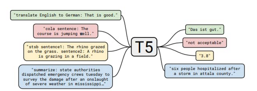
Over the  years, businesses have increasingly used Dataflow for its ability to pre-process stream and/or batch data for machine learning. Some success stories include Harambee, Monzo, Dow Jones, and Fluidly.A growing number of other customers are using machine learning inference in Dataflow pipelines to extract insights from data. Customers have the choice of either using ML models loaded into the Dataflow pipeline itself, or calling ML APIs provided by Google Cloud. As these use cases develop, there are some common patterns being established which will be explored in this series of blog posts. In part I of this series, we’ll explore the process of providing a model with data and extracting the resulting output, specifically:Local/remote inference efficiency patternsBatching patternSingleton model patternMulti-model inference pipelinesData branching to get the data to multiple modelsJoining results from multiple branches Although the programming language used throughout this blog is Python, many of the general design patterns will be relevant for other languages supported by Apache Beam pipelines. This also holds true for the ML framework; here we are using TensorFlow but many of the patterns will be useful for other frameworks like PyTorch and XGBoost. At its core, this is about delivering data to a model transform and the post processing of that data downstream.To make the patterns more concrete for the local model use case, we will make use of the open source “Text-to-Text Transfer Transformer” (T5) model which was published in “Exploring the Limits of Transfer Learning with a Unified Text-to-Text Transformer”. The paper presents a large-scale empirical survey to determine which transfer learning techniques for language modelling work best, and applies these insights at scale to produce a model that achieves state-of-the-art results on numerous NLP tasks.In the sample code, we made use of the “Closed-Book Question Answering” ability, as explained in the T5 blog;”…In our Colab demo and follow-up paper, we trained T5 to answer trivia questions in a more difficult ‘closed-book’ setting, without access to any external knowledge. In other words, in order to answer a question T5 can only use knowledge stored in its parameters that it picked up during unsupervised pre-training. This can be considered a constrained form of open-domain question answering.” For example, we ask the question, “How many teeth does a human have?” and the model returns with “20 primary.” The model is well suited for our discussion, as in its largest incarnation it has over 11 billion parameters and is over 25 Gigabytes in size, which necessitates following the good practices described in this blog. Setting up the T5 ModelThere are several sizes of the T5 model, in this blog we will make use of  small and XXL sizes. Given the very large memory footprint needed by the XXL mode (25 GB for the save model files), we recommend working with the small version of the model when exploring most of the code samples below. You can download instructions from the T5 team in this colab. For the final code sample in this blog, you’ll need the XXL model, we recommend running that code via python command on a machine with 50+ GB of memory.The default for the T5 model export is to have an inference batch size of 1. For our purposes, we’ll need this to be set to 10 by adding –batch_size=10 as seen in the code sample below.Batching patternA pipeline can access a model either locally (internal to the pipeline) or remotely (external to the pipeline).  In Apache Beam, a data processing task is described by a pipeline, which represents a directed acyclic graph (DAG) of transformations (PTransforms) that operate on collections of data (PCollections). A pipeline can have multiple PTransforms, which can execute user code defined in do-functions (DoFn, pronounced as do-fun) on elements of a PCollection. This work will be distributed across workers by the Dataflow runner, scaling out resources as needed.Inference calls are made within the DoFn. This can be through the use of functions that load models locally or via a remote call, for example via HTTP, to an external API endpoint. Both of these options require specific considerations in their deployment, and these patterns are explored below.Inference flowBefore we outline the pattern, let’s look at the various stages of making a call to an inference function within our DoFn.Convert the raw data to the correct serialized format for the function we are calling. Carry out any preprocessing required.Call the inference function:In local mode: Carry out any initialization steps needed (for example loading the model). Call the inference code with the serialized data.In remote mode, the serialized data is sent to an API endpoint, which requires establishing a connection, carrying out authorization flows, and finally sending the data payload.Once the model processes the raw data, the function returns with the serialized result.Our DoFn can now deserialize the result ready for postprocessing.The administration overhead of initializing the model in the local case, and the connection/auth establishment in the remote case, can become significant parts of the overall processing. It is possible to reduce this overhead by batching before calling the inference function. Batching allows us to amortize the admin costs across many elements, improving efficiency. Below, we discuss several ways you can achieve batching with Apache Beam, as well as ready made implementations of these methods.Batching through Start/Finish bundle lifecycle eventsWhen an Apache Beam runner executes pipelines, every DoFn instance processes zero or more “bundles” of elements. We can use DoFn’s life cycle events to initialize resources shared between bundles of work. The helper transform BatchElements leverages start_bundle and finish_bundle methods to regroup elements into batches of data, optimizing the batch size for amortized processing.  Pros:  No shuffle step is required by the runner. Cons: Bundle size is determined by the runner. In batch mode, bundles are large, but in stream mode bundles can be very small.Note: BatchElements attempts to find optimal batch sizes based on runtime performance. “This transform attempts to find the best batch size between the minimum and maximum parameters by profiling the time taken by (fused) downstream operations. For a fixed batch size, set the min and max to be equal.” (Apache Beam documentation) In the sample code we have elected to set both min and max for consistency.In the example below, sample questions are created in a batch ready to send to the T5 model:Batching through state and timers The state and timer API is the primitives within Apache Beam which other higher level primitives like windows are built on. Some of the public batching mechanisms used for making calls to Google Cloud APIs like the Cloud Data Loss Prevention API via Dataflow templates, rely on this mechanism. The helper transform GroupIntoBatches leverages the state and timer API to group elements into batches of desired size. Additionally it is key-aware and will batch elements within a key. Pros: Fine-grained control of the batch, including the ability to make data driven decisions.Cons: Requires shuffle.CombinersApache Beam Combiner API allows elements to be combined within a PCollection, with variants that work on the whole PCollection or on a per key basis. As Combine is a common transform, there are a lot of examples of its usage in the core documents.Pros: Simple APICons: Requires shuffle. Coarse-grained control of the output.With these techniques, we will now have a batch of data to use with the model, including the initialization cost, now amortized across the batch. There is more that can be done to make this work efficient, particularly for large models when dealing with local inference. In the next section we will explore inference patterns. Remote/local inferenceNow that we have a batch of data that we would like to send to a model for inference, the next step will depend on whether the inference will be local or remote. Remote inferenceIn remote inference, a remote procedure call is made to a service outside of the Dataflow pipeline. For a custom built model, the model could be hosted, for example on a Kubernetes cluster or through a managed service such as Google Cloud AI Platform Prediction. For pre-built models which are provided as a service, the call will be to the service endpoint, for example Google Cloud Document AI. The major advantage of using remote inference is that we do not need to assign pipeline resources to loading the model, or take care of versions.Factors to consider with remote calls:Ensure that the total batch size is within the limits provided by the service. Ensure that the endpoint being called is not overwhelmed, as Dataflow will spin up resources to deal with the incoming load. You can limit the total number of threads being used in the calls by several options:Set the max_num_workers value within the pipeline options.If required, make use of worker process/thread control (discussed in more depth later in this blog).In circumstances when remote inference is not possible, the pipeline will also need to deal with actions like loading the model and sharing that model across multiple threads. We’ll look at these patterns next.  Local inferenceLocal inference is carried out by loading the model into memory. This heavy initialization action, especially for larger models, can require more than just the Batching pattern to perform efficiently. As discussed before, the user code encapsulated in the DoFn is called against every input. It would be very inefficient, even with batching, to load the model on every invocation of the DoFn.process method.In the ideal scenario the model lifecycle will follow this pattern:Model is loaded into memory by the transformation used for prediction work.Once loaded, the model serves data, until an external life cycle event forces a reload.Part of the way we reach this pattern is to make use of the shared model pattern, described in detail below.Singleton model (shared.py)The shared model pattern allows all threads from a worker process to make use of a single model by having only one instance of the model loaded into memory per process.  This pattern is common enough that the shared.py utility class has been made available in Apache Beam since version 2.24.0. End-to-end local inference example with T5 modelIn the below code example, we will apply both the batching pattern as well as the shared model pattern to create a pipeline that makes use of the T5 model to answer general knowledge questions for us.In the case of the T5 model, the batch size we specified requires the array of data that we send to it to be exactly of length 10. For the batching, we will make use of the BatchElements utility class. An important consideration with BatchElements is that the batch size is a target, not a guarantee of size. For example, if we have 15 examples, then we might get two batches; one of 10 and one of 5. This is dealt with in the processing functions shown in the code.Please note the inference call is done directly via model.signatures as a simple way to show the application of the shared.py pattern, which is to load a large object once and then reuse.  (The code lab t5-trivia shows an example of wrapping the predict function).Note: Determining the optimum batch size is very workload specific and would warrant an entire blog discussion on its own. Experimentation as always the key for understanding the optimum size/latency.Note: If the object you are using for shared.py can not be safely called from multiple threads, you can make use of a locking mechanism. This will limit parallelism on the worker, but the trade off may still be useful depending on the size / initialization cost of loading the model. Running the code sample will produce the following output (when using the small T5 model):Worker thread/process control (advanced) With most models, the techniques we have described so far will be enough to run an efficient pipeline. However, in the case of extremely large models like the T5 XXL, you will need to provide more hints to the runner to ensure that the workers have enough resources to load the model. We are working on improving this and we will remove the needs for these parameters eventually. But until then, use this if your models need it.A single runner is capable of running many processes and threads on a worker, as shown in the diagram below:The parameters detailed below are those that can be used with the Dataflow Runner v2. Runner v2 is currently available using the flag –experiments=use_runner_v2.To ensure that the total_memory/num processes are at a ratio that can support large models, these values will need to be set as follows:If using the shared.py pattern, the model will be shared across all threads but not across processes. If not using the shared.py pattern and the model is loaded, for example, within the @setup DoFn lifecycle event, then make use of number_of_worker_harness_threads to match the memory of the worker.Multiple-model inference pipelinesIn the previous set of patterns, we covered the mechanics of enabling efficient inference. In this section, we will look at some functional patterns which allow us to leverage the ability to create multiple inference flows within a single pipeline. Pipeline branchesA branch allows us to flow the data in a PCollection to different transforms. This allows multiple models to be supported in a single pipeline, enabling useful tasks like: A/B testing using different versions of a model. Having different models produce output from the same raw data, with the outputs fed to a final model.Allowing a single data source to be enriched and shaped in different ways for different use cases with separate models, without the need for multiple pipelines.In Apache Beam, there are two easy options to create a branch in the inference pipeline. One is by applying multiple transformations to a PCollection:The other uses multi-output transforms:Using T5 and the branch pattern As we have multiple versions of our T5 model (small and XXL), we can run some tests which branch the data, carry out inference on different models, and join the data back together to compare the results. For this experiment, we will use a more ambiguous question of the form. “Where does the name {first name} come from.” The intent of the question is to determine the origins of the first names. Our assumption is that the XXL model will do better with these names than the small model. Before we build out the example, we first need to show how to enhance the previous code to give us a way to bring the results of two separate branches back together. Using the previous code, the predict function can be changed by merging the questions with the inferences via zip().Building the pipelineThe pipeline flow is as follows:Read in the example questions.Send the questions to the small and XXL versions of the model via different branches.Join the results back together using the question as the key.Provide simple output for visual comparison of the values.Note: To run this code sample with the  XXL model and the directrunner, you will need a machine with a minimum of 60GB of memory. You can also of course run this example code with any of the other sizes that fall between the small to XXL which will have a lower memory requirement.The output is shown below.As we can see, the larger XXL model did a lot better than the small version of the model. This makes sense as the additional parameters allow the model to store more world knowledge. This result is confirmed by findings of https://arxiv.org/abs/2002.08910″. Importantly, we now have a tuple which contains the predictions from both of the models which can be easily used downstream. Below we can see the shape of the graph produced by the above code when run on the Dataflow Runner.Note: To run the sample on the Dataflow runner, please make use of a setup.py file with the install_requires parameters as below, the tensorflow-text is important as the T5 model requires the library even though it is not used directly in the code samples above.install_requires=[‘t5==0.7.1′, ‘tensorflow-text==2.3.0′, ‘tensorflow==2.3.1′]A high memory machine will be needed with the XXL model, the pipeline above was run with configuration:machine_type = custom-1-106496-extnumber_of_worker_harness_threads = 1experiment = use_runner_v2As the XXL model is > 25 Gig in size, with the load operation taking more than 15 mins. To reduce this load time, use a custom container.The predictions with the XXL model can take many minutes to complete on a CPU.Batching and branching:Joining the results:ConclusionIn this blog, we covered some of the patterns for running remote/local inference calls, including; batching, the singleton model pattern, and understanding the processing/thread model for dealing with large models. Finally, we touched on how the easy creation of complex pipeline shapes can be used for more advanced inference pipelines. To learn more, review the Dataflow documentation.
Quelle: Google Cloud Platform

Get to know Workflows, Google Cloud’s serverless orchestration engine

Whether your company is processing e-commerce transactions, producing goods or delivering IT services, you need to manage the flow of work across a variety of systems. And while it’s possible to manage those workflows manually or with general-purpose tools, doing so is much easier with a purpose-built product. Google Cloud has two workflow tools in its portfolio: Cloud Composer and the new Workflows. Introduced in August, Workflows is a fully managed workflow orchestration product running as part of Google Cloud. It’s fully serverless and requires no infrastructure management.In this article we’ll discuss some of the use cases that Workflows enables, its features, and tips on using it effectively.A sample workflowFirst, consider the following workflow for generating an invoice:A common way to orchestrate these steps is to call API services based on Cloud Functions, Cloud Run or a public SaaS API, e.g. SendGrid, which sends an e-mail with our PDF attachment. But real-life scenarios are typically much more complex than the example above and require continuous tracking of all workflow executions, error handling, decision points and conditional jumps, iterating arrays of entries, data conversions and many other advanced features. Which is to say, while technically you can use general-purpose tools to manage this process, it’s not ideal. For example, let’s consider some of the challenges you’d face processing this flow with an event-based compute platform like Cloud Functions. First, the max duration of a Cloud Function run is nine minutes, but workflows—especially those involving human interactions—can run for days; your workflow may need more time to complete, or you may need to pause in between steps when polling for a response status. Attempting to chain multiple Cloud Functions together with for instance, Pub/Sub also works, but there’s no simple way to develop or operate such a workflow. First, in this model it’s very hard to associate step failures with workflow executions, making troubleshooting very difficult. Also, understanding the state of all workflow executions requires a custom-built tracking model, further increasing the complexity of this architecture. In contrast, workflow products provide support for exception handling and give visibility on executions and the state of individual steps, including successes and failures. Because the state of each step is individually managed, the workflow engine can seamlessly recover from errors, significantly improving reliability of the applications that use the workflows. Lastly, workflow products often come with built-in connectors to popular APIs and cloud products, saving time and letting you plug into existing API interfaces. Workflow products on Google CloudGoogle Cloud’s first general purpose workflow orchestration tool was Cloud Composer.Based on Apache Airflow, Cloud Composer is great for data engineering pipelines like ETL orchestration, big data processing or machine learning workflows, and integrates well with data products like BigQuery or Dataflow . For example, Cloud Composer is a natural choice if your workflow needs to run a series of jobs in a data warehouse or big data cluster, and save results to a storage bucket.However, if you want to process events or chain APIs in a serverless way—or have workloads that are bursty or latency-sensitive—we recommend Workflows. Workflows scales to zero when you’re not using it, incurring no costs when it’s idle. Pricing is based on the number of steps in the workflow, so you only pay if your workflow runs. And because Workflows doesn’t charge based on execution time, if a workflow pauses for a few hours in between tasks, you don’t pay for this either. Workflows scale up automatically with very low startup time and no “cold start” effect. Also, it transitions quickly between steps, supporting latency-sensitive applications. Workflows use casesWhen it comes to the number of processes and flows that Workflows can orchestrate, the sky’s the limit. Let’s take a look at some of the more popular use cases. Processing customer transactionsImagine you need to process customer orders and, in the case that an item is out of stock, trigger an inventory refill from an external supplier. During order processing you also want to notify your sales reps about large customer orders. Sales reps are more likely to react quickly if they get such notifications using Slack. Here is an example workflow diagram.The workflow above orchestrates calls to Google Cloud’s Firestore as well as external APIs including Slack, SendGrid or the inventory supplier’s custom API. It passes the data between the steps and implements decision points that execute steps conditionally, depending on other APIs’ outputs. Each workflow execution—handling one transaction at a time—is logged so you can trace it back or troubleshoot it if needed. The workflow handles necessary retries or exceptions thrown by APIs, thus improving the reliability of the entire application. Processing uploaded filesAnother case you may consider is a workflow that tags files that users have uploaded based on file contents. Because users can upload text files, images or videos, the workflow needs to use different APIs to analyze the content of these files. In this scenario, a Cloud function is triggered by a Cloud Storage trigger. Then, the function starts a workflow using the Workflows client library, and passes the file path to the workflow as an argument. In this example, a workflow decides which API to use depending on the file extension, and saves a corresponding tag to a Firestore database.Workflows under the hoodYou can implement all of these use cases out of the box with Workflows. Let’s take a deeper look at some key features you’ll find in Workflows. StepsWorkflows handles sequencing of activities delivered as ‘steps’. If needed, a workflow can also be configured to pause between steps without generating time-related charges.In particular, you can orchestrate practically any API that is network-reachable and follows HTTP as a workflow step. You can make a call to any internet-based API, including SaaS APIs or your private endpoints, without having to wrap such calls in Cloud Functions or Cloud Run.AuthenticationWhen making calls to Google Cloud APIs, e.g., to invoke a Cloud function or read data from Firestore, Workflows uses built-in IAM authentication. As long as your workflow has been granted IAM permission to use a particular Google Cloud API, you don’t need to worry about authentication protocols.Communication between workflow stepsMost real-life workflows require that steps communicate with one another. Workflows supports built-in variables that steps can use to pass the result of their work to a subsequent step. Automatic JSON conversionAs JSON is very common in API integrations, Workflows automatically converts API JSON responses to dictionaries, making it easy for the following steps to access this information. Rich expression languageWorkflows also comes with a rich expression language supporting arithmetic and logical operators, arrays, dictionaries and many other features. The ability to perform basic data manipulations directly in the workflow further simplifies API integrations. Because Workflows accepts runtime arguments, you can use a single workflow to react to different events or input data.Decision pointsWith variables and expressions, we can implement another critical component of most workflows: decision points. Workflows can use custom expressions to decide whether to jump to another part of the workflow or conditionally execute a step. Conditional step executionFrequently used parts of the logic can be coded as a sub-workflow and then called as a regular step, working similarly to routines in many programming languages.Sometimes, a step in a workflow fails, e.g., due to a network issue or because a particular API is down. This, however, shouldn’t immediately make the entire workflow execution fail. Workflows avoids that problem with a combination of configurable retries and exception handling that together allow a workflow to react appropriately to an error returned by the API call.All features above are configurable as part of the Workflows source code. You can see practical examples of these configurationshere. Get started with Workflows todayWorkflows is a powerful new addition to Google Cloud’s application development and management toolset, and you can try it out immediately on all your projects. Have a look at theWorkflows site or go right ahead to theCloud Console to build your first workflow. Workflows comes with a free tier so you can give it a try at no cost. Also, watch out for exciting Workflows announcements coming soon!Happy orchestrating! :)
Quelle: Google Cloud Platform

Getting higher MPI performance for HPC applications on Google Cloud

Most High Performance Computing (HPC) applications such as large-scale engineering simulations, molecular dynamics, and genomics, run on supercomputers or HPC clusters on-premises. Cloud is emerging as a great option for these workloads due to its elasticity, pay per use, and the lower associated maintenance cost.Reducing Message Passing Interface (MPI) latency is one critical element of delivering HPC application performance and scalability. We recently introduced several features and tunings that make it easy to run MPI workloads and achieve optimal performance on Google Cloud. These best practices reduce MPI latency, especially for applications that depend on small messages and collective operations. These best practices help optimize Google Cloud systems and networking infrastructure to improve MPI communication over TCP without requiring major software changes or new hardware support. With these best practices, MPI ping-pong latency falls into single-digits of microseconds (μs), and small MPI messages are delivered in 10μs or less. In the figure below, we show how progressive optimizations lowered one-way latency from 28 to 8μs with a test setup on Google Cloud.Improved MPI performance translates directly to improved application scaling, expanding the set of workloads that run efficiently on Google Cloud. If you plan to run MPI workloads on Google Cloud, use these practices to get the best possible performance. Soon, you will be able to use the upcoming HPC VM Image to easily apply these best practices and get the best out-of-the-box performance for your MPI workloads on Google Cloud.1. Use Compute-optimized VMsCompute-optimized (C2) instances have a fixed virtual-to-physical core mapping and expose NUMA architecture to the guest OS. These features are critical for performance of MPI workloads. They also leverage second Generation Intel Xeon Scalable Processors (Cascade Lake), which can provide up to a 40% improvement in performance compared to previous generation instance types due to their support for a higher clock speed of 3.8 GHz, and higher memory bandwidth. C2 VMs also support vector instructions (AVX2, AVX512). We have noticed significant performance improvement for many HPC applications when they are compiled with AVX instructions. 2. Use compact placement policy A placement policy gives you more control over the placement of your virtual machines within a data center. A compact placement policy ensures instances are hosted in nodes nearby on the network, providing lower latency topologies for virtual machines within a single availability zone. Placement policy APIs currently allow creation of up to 22 C2 VMs.3. Use Intel MPI and collective communication tuningsFor the best MPI application performance on Google Cloud, we recommend the use of Intel MPI 2018. The choice of MPI collective algorithms can have a significant impact on MPI application performance and Intel MPI allows you to manually specify the algorithms and configuration parameters for collective communication. This tuning is done using mpitune and needs to be done for each combination of the number of VMs and the number of processes per VM on C2-Standard-60 VMs with compact placement policies. Since this takes a considerable amount of time, we provide the recommended Intel MPI collective algorithms to use in the most common MPI job configurations.For better performance of scientific computations, we also recommend use of Intel Math Kernel Library (MKL).4. Adjust Linux TCP settingsMPI networking performance is critical for tightly coupled applications in which MPI processes on different nodes communicate frequently or with large data volume. You can tune these network settings for optimal MPI performance.Increase tcp_mem settings for better network performanceUse network-latency profile on CentOS to enable busy polling5. System optimizationsDisable Hyper-ThreadingFor compute-bound jobs in which both virtual cores are compute bound, Intel Hyper-Threading can hinder overall application performance and can add nondeterministic variance to jobs. Turning off Hyper-Threading allows more predictable performance and can decrease job times. Review security settingsYou can further improve MPI performance by disabling some built-in Linux security features. If you are confident that your systems are well protected, you can evaluate disabling the following security features as described in Security settings section of the best practices guide:Disable Linux firewallsDisable SELinuxTurn off Spectre and Meltdown MitigationNow let’s measure the impact  In this section we demonstrate the impact of applying these best practices through application-level benchmarks by comparing the runtime with select customers’ on-prem setups: (i) National Oceanic and Atmospheric Administration (NOAA) FV3GFS benchmarksWe measured the impact of the best practices by running the NOAA FV3GFS benchmarks with the C768 model and 104 C2-Standard-60 Instances (3,120 physical cores). The expected runtime target, based on on-premise supercomputers, was 600 seconds. Applying these best practices provided a 57% improvement compared to baseline measurements—we were able to run the benchmark in 569 seconds on Google Cloud (faster than the on-prem supercomputer).(ii) ANSYS LS-DYNA engineering simulation softwareWe ran the LS-DYNA 3 cars benchmark using C2-Standard-60 instances, AVX512 instructions and a compact placement policy. We measured scaling from 30 to 120 MPI ranks (1-4 VMs) . By implementing these best practices, we achieved on-par or better runtime performance on Google Cloud in many cases when compared with the customer’s on-prem setup with specialized hardware.There is more: easy and efficient application of best practices To simplify deployment of these best practices, we created an HPC VM Image based on CentOS 7 and that makes it easy to apply these best practices and get the best out-of-the-box performance for your MPI workloads on Google Cloud. You can also apply the tunings to your own image, using the bash and Ansible scripts published in the Google HPC-Tools Github repository or by following the best practice guide.To request access to HPC VM Image, please sign up via this form. We recommend benchmarking your applications to find the most efficient or cost-effective configuration.Applying these best practices can improve application performance and reduce cost. To further reduce and manage costs, we also offer automatic sustained use discounts, transparent pricing with per-second billing, and preemptible VMs that are discounted up to 80% versus regular instance types.Visit our website to get started with HPC on Google Cloud today.
Quelle: Google Cloud Platform