Future-proofing your business with Google Cloud and SAP

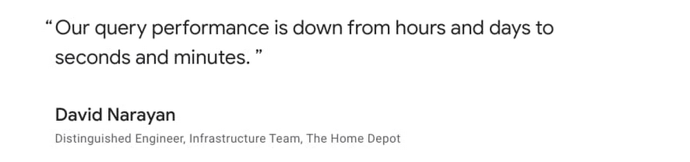
Things are changing fast for just about every business. Many are fundamentally shifting how they operate and how they serve their customers. Add in a global pandemic, and even organizations that are used to change are managing unprecedented shifts.Businesses running on SAP applications know this all too well. Some are adapting to shifting market conditions while others are operating every day like Black Friday. For SAP enterprises running on-premises or in co-location data centers, the imperative of the cloud is in the fore more than ever. As SAP’s SAPPHIRE NOW digital events kick off this week, we’re sharing the latest on how Google Cloud is helping SAP customers digitally transform their businesses in the short and long term.SAP customers are benefiting from the combined power of Google Cloud and SAPGoogle Cloud and SAP continue working together to help customers adopt a cloud strategy and build robust, flexible and innovative IT systems that will sustain them into the future. SAP recently announced the first ever SAP data center powered by Google Cloud infrastructure. Now operational in Frankfurt, Germany, this data center will allow SAP’s customers to enjoy all the benefits of Google Cloud’s solid and reliable cloud platform on Google Cloud infrastructure that is exclusive only to SAP applications. SAP can run customer workloads and administer capacity and services exclusively for those customers without the risk of being impacted by any external influence, while providing a secure environment based on SAP’s strict specifications regarding data protection requirements and compliance standards. There are more ways we’re innovating on behalf of our joint customers outside the data center. AutoML Vision is an intelligent, AI-powered solution that lets manufacturers automate the visual quality control process. Instead of relying on manual inspections—sometimes conducted under challenging conditions—customers such as AES and Kaeser Kompressoren are leveraging AutoML Vision, which is embedded into manufacturing and business workflows built around SAP, to perform quality controls efficiently and at any production stage. For manufacturing customers that have begun their Industry 4.0 journey, integrating AI-powered visual inspection is a critical piece that’s empowering them to achieve digital transformation.Getting to the cloud for business agility and insightsCurrent market conditions are creating an even greater need for SAP customers to take advantage of cloud agility and innovation. Tory Burch was able to complete SAP S/4HANA development in 16 weeks and deployment in six weeks on Google Cloud. Carrefour Spain deployed SAP HANA in production in 15 weeks. And they’re not alone. SAP customers report a 65% reduction in staff time to deploy/migrate SAP applications to Google Cloud. Our automated templates plus capabilities such as Migrate for Compute Engine offer significant support for customers in speeding deployments. To help SAP customers further simplify their cloud journeys, Google Cloud offers the Cloud Acceleration Program (CAP), a first-of-its-kind initiative empowering customers with solutions, guidance, and incentives from Google Cloud and our expert partner community. Customers receive access to expert capabilities for migration, implementation optimization plus deeper capabilities in the areas of analytics and machine learning. Google Cloud is also providing CAP participants with upfront financial incentives to defray infrastructure costs for SAP cloud migrations and help customers ensure that duplicate costs are not incurred during migration. New Google Cloud and partner capabilities for SAP customersOne key area where we continue to invest is certifications to drive more workloads, like OLTP and OLAP. This allows customers to use our VMs for more varied workloads and provides more throughput and better processing—without customers having to upgrade, move, or pay more. These performance bumps are simply part of customers’ existing subscriptions. Recently updated SAP HANA certifications include Google Cloud Compute Engine’s N2 family of VM instances, based on Intel Cascade Lake CPU platform. These new N2 VMs deliver two big benefits for our customers: Performance improvements for SAP HANA workloads. In SAP certification tests we have seen up to an 18% increase in performance for OLAP scenarios.Alignment to SAP HANA Enterprise Edition licensing’s 64GB memory unit metric. This enables customers to ‘right size’ their Google Cloud VMs to match their SAP HANA licenses—no need for VM capacity that they can’t use. In addition, for larger SAP HANA deployments, we recently announced the OLAP Scale-up certification for our M2 family of Compute Engine VM instances for SAP HANA with 6TB of memory. This gives customers increased options for running OLAP scenarios such as SAP HANA data warehouse and SAP BW/HANA.We’ve also been making improvements for SAP Netweaver deployments. A key example is the addition of new SAP NetWeaver certifications for the AMD-based N2D family of Compute Engine VM instances. The N2D instances give customers a benchmark-setting high-performance solution—up to 30% faster than prior Google Cloud offerings based on our SAPS benchmark testing, and at a lower-cost. This offers customers optionality and flexibility of choice for deploying SAP NetWeaver applications or SAP application servers alongside their SAP HANA deployments. One additional certification to mention is SAP Adaptive Server Enterprise (ASE) Database 16.0. This latest version of ASE is now certified on Google Cloud both for SAP NetWeaver based application deployments and also for customers who build applications on SAP ASE as a general purpose database.Customers also will soon be able to leverage a Google Cloud connector for SAP Landscape Management (LaMa) so they can automate and centralize the management, operations and lifecycle of their SAP landscape. The adapter will interface with Compute Engine and Cloud Storage operations so customers can manage their deployments on Google Cloud using SAP LaMa.Additionally, premium support for your enterprise and mission critical needs is now available, including a pilot program with supplementary support of SAP customers. The program layers Google Cloud premium support on top of the stellar support that SAP provides, and will roll out more broadly in the coming months.We’ve also strengthened our SAP partner ecosystem to ensure that our customers running SAP applications have access to the right tools and services. These include the following:Actifiooffers data protection capabilities for mission critical workloads such as SAP on Google Cloud. These highly efficient backup and recovery capabilities insure protection while minimizing required compute, bandwidth and storage. Avantra has tailored their solution for monitoring and managing SAP applications specifically for Google Compute Engine, enabling in-depth automation of SAP management and operations.Data management and integration partners—Informatica, Qlik, Datavard,and Software AG offer a robust set of tools and solutions to extract data from SAP systems including ECC, S/4 and BW into BigQuery as the target data warehouse. These solutions help aggregate data from SAP and non-SAP systems into a centralized, highly scalable data warehouse where customers can take advantage of Google Cloud’s smart analytics and machine learning services. Customers can get started quickly leveraging Google Cloud Marketplace solutions such as the Informatica Intelligent Cloud Services solution. IBM Power Systems is available for large enterprises that want to take advantage of these systems along with Google Cloud for IaaS and VM needs. NetApp for enterprise storage, delivering NetApp Cloud Volumes Service for Google Cloud—This is a fully managed file service integrated into Google Cloud with multi-protocol support, dynamic performance and high availability. The service is certified for use with SAP HANA scale up deployments on all Compute Engine VM instances that are certified for SAP HANA on Google Cloud. When Conrad Electronic, a B2B and B2C technology and electronics goods supplier, realized it could use its vast data set to optimize the company’s processes and offer more products and services with the help of Google Cloud, it decided to keep using its legacy SAP systems but consolidate all data on BigQuery. This allows Conrad to generate better, more insightful reports, analyze information faster, and automate more processes. “With BigQuery, we see all of our processes from start to finish, and every stage in between,” says Aleš Drábek, Chief Digital and Disruption Officer at Conrad Electronic. “We identify aspects to improve and can get the detail we need to improve them. Our legacy systems gave an overview on part of the process. Now we can see the whole thing.”Keeping the lights on and lighting the way forward for our customers As one of the largest healthcare organizations in the U.S., Cardinal Healthhas not been immune to market-related pressures. After migrating its SAP environment for its pharmaceutical business to Google Cloud in late 2019—which included more than 400 servers, 30 applications, and 150 integrations—Cardinal Health gained the scalability needed to manage demand spikes, full transparency into its systems as well as improved high availability and disaster recovery. The need to adapt to demand spikes and create supply chain transparency goes beyond healthcare. The Home Depot manages data from its SAP systems and other sources and empower its associates with Google Cloud, keeping 50,000+ items stocked in store at over 2,000 locations, monitoring online applications, or offering relevant call center information. While THD’s legacy data warehouse contained 450 terabytes of data, the BigQuery enterprise data warehouse they now use has over 15 petabytes. That means better decision-making by utilizing new datasets like website clickstream data and by analyzing additional years of data.As SAP customers begin and continue their cloud journeys, Google Cloud is committed to being there to simplify and optimize their move and ensure they have ready access to critical cloud native technologies. To see more work that we’ve done with SAP and SAP customers, visit our solution site, and check out our customer video testimonials.
Quelle: Google Cloud Platform

What a trip! Measuring network latency in the cloud

A common question for cloud architects is “Just how quickly can we exchange a request and a response between two endpoints?” There are several tools for measuring round-trip network latency, namely ping, iperf, and netperf, but because they’re not all implemented and configured the same, different tools can return different results. And in most cases, we believe netperf returns the more representative answer to the question—you just need to pay attention to the details. Google has lots of practical experience in latency benchmarking, and in this blog, we’ll share techniques jointly developed by Google and researchers at Southern Methodist University’s AT&T Center for Virtualization to inform your own latency benchmarking before and after migrating workloads to the cloud. We’ll also share our recommended commands for consistent, repeatable results running both intra-zone cluster latency and inter-region latency benchmarks.Which tools and whyAll the tools in this area do roughly the same thing: measure the round trip time (RTT) of transactions. Ping does this using ICMP packets, and several tools based on ping such as nping, hping, and TCPing perform the same measurement using TCP packets. For example, using the following command, ping sends one ICMP packet per second to the specified IP address until it has sent 100 packets.ping <ip.address> -c 100Network testing tools such as netperf can perform latency tests plus throughput tests and more. In netperf, the TCP_RR and UDP_RR (RR=request-response) tests report round-trip latency. With the -o flag, you can customize the output metrics to display the exact information you’re interested in. Here’s an example of using the test-specific -o flag so netperf outputs several latency statistics:netperf -H <ip.address> -t TCP_RR —   -o min_latency,max_latency,mean_latency*Note: this uses global options: -H for remote-host and -t for test-name with a test-specific option -o for output-selectors. Example.As described in a previous blog post, when we run latency tests at Google in a cloud environment, our tool of choice is PerfKit Benchmarker (PKB). This open-source tool allows you to run benchmarks on various cloud providers while automatically setting up and tearing down the virtual infrastructure required for those benchmarks. Once you set up PerfKit Benchmarker, you can run the simplest ping latency benchmark or a netperf TCP_RR latency benchmark using the following commands:These commands run intra-zone latency benchmarks between two machines in a single zone in a single region. Intra-zone benchmarks like this are useful for showing very low latencies, in microseconds, between machines that work together closely. We’ll get to our favorite options and method to run these commands later in this post.Latency discrepanciesLet’s dig into the details of what happens when PerfKit Benchmarker runs ping and netperf to illustrate what you might experience when you run such tests.Here, we’ve set up two c2-standard-16 machines running Ubuntu 18.04 in zone us-east1-c, and we’ll use internal ip addresses to get the best results. If we run a ping test with default settings and set the packet count to 100, we get the following results:By default, ping sends out one request each second. After 100 packets, the summary reports that we observed an average latency of 0.146 milliseconds, or 146 microseconds.For comparison, let’s run netperf TCP_RR with default settings for the same amount of packets.Here, netperf reports an average latency of 66.59 microseconds. The ping average latency reported is ~80 microseconds different than the netperf one; ping reports a value more than twice that of netperf! Which test can we trust?To explain, this is largely an artifact of the different intervals the two tools used by default. Ping uses an interval of 1 transaction per second while netperf issues the next transaction immediately when the previous transaction is complete. Fortunately, both of these tools allow you to manually set the interval time between transactions, so you can see what happens when adjusting the interval time to match. For ping, use the -i flag to set the interval, given in seconds or fractions of a second. On Linux systems, this has a granularity of 1 millisecond, and rounds down. For example, if you use an interval of 0.00299 seconds, this rounds down to 0.002 seconds, or 2 milliseconds. If you request an interval smaller than 1 millisecond, ping rounds down to 0 and sends requests as quickly as possible. You can start ping with an interval of 10 milliseconds using:$ ping <ip.address> -c 100 -i 0.010For netperf TCP_RR, we can enable some options for fine-grained intervals by compiling it with the –enable-spin flag. Then, use the -w flag, which sets the interval time, and the -b flag, which sets the number of transactions sent per interval. This approach allows you to set intervals with much finer granularity, by spinning in a tight loop until the next interval instead of waiting for a timer; this keeps the cpu fully awake. Of course, this precision comes at the cost of much higher CPU utilization as the CPU is spinning while waiting. *Note: Alternatively, you can set less fine-grained intervals by compiling with the –enable-intervals flag. Use of the -w and -b options requires building netperf with either the –enable-intervals or –enable-spin flag set.The tests here are performed with the –enable-spin flag set. You can start netperf with an interval of 10 milliseconds using:$ netperf -H <ip.address> -t TCP_RR -w 10ms -b 1 —   -o min_latency,max_latency,mean_latencyNow, after aligning the interval time for both ping and netperf to 10 milliseconds, the effects are apparent:ping:netperf:By setting the interval of each to 10 milliseconds, the tests now report an average latency of 81 microseconds for ping and 94.01 microseconds for netperf, which are much more comparable.You can illustrate this effect more clearly by running more tests with ping and netperf TCP_RR over a range of varied interval times ranging from 1 microsecond to around ~1 second and plotting the results.The latency curves from both tools look very similar. For intervals below ~1 millisecond, round-trip latency remains relatively constant around 0.05-0.06 milliseconds. From there, latency steadily increases.TakeawaysSo which tool’s latency measurement is more representative—ping or netperf—and when does this latency discrepancy actually matter?Generally, we recommend using netperf over ping for latency tests. This isn’t due to any lower reported latency at default settings, though. As a whole, netperf allows greater flexibility with its options and we prefer using TCP over ICMP. TCP is a more common use case and thus tends to be more representative of real-world applications. That being said, the difference between similarly configured runs with these tools is much less across longer path lengths.Also, remember that interval time and other tool settings should be recorded and reported when performing latency tests, especially at lower latencies, because these intervals make a material difference.To run our recommended benchmark tests with consistent, repeatable results, try the following:For intra-zone cluster latency benchmarking:This benchmark uses an instance placement policy which is recommended for workloads which benefit from machines with very close proximity to each other.For inter-region latency benchmarking:Notice that the netperf TCP_RR benchmarks run with no additional interval setting. This is because by default netperf inserts no added intervals between request/response transactions; this induces more accurate and consistent results.Note: This latest netperf intra-zone cluster latency result benefits from controlling any added intervals in the test and from using a placement group.What’s nextIn our next network performance benchmarking post, we’ll get into the details about how to use the new public-facing Google Cloud global latency dashboard to better understand the impact of cloud migrations on your workloads. Also, be sure to check out our PerfKit Benchmarker white paper and the PerfKit Benchmarker tutorials for step-by-step instructions running networking benchmark experiments!Special thanks to Mike Truty, Technical Curriculum Lead, Google Cloud Learning for his contributions.
Quelle: Google Cloud Platform

Introducing Spark 3 and Hadoop 3 on Dataproc image version 2.0

Dataproc makes open source data and analytics processing fast, easy, and more secure in the cloud. Dataproc provides fully configured autoscaling clusters in around 90 seconds on custom machine types. This makes Dataproc an ideal way to experiment with and test the latest functionality from the open source ecosystem. Dataproc provides image versions that align with bundles of core software that typically come on Hadoop and Spark clusters. Dataproc optional components can extend this bundle to include other popular open source technologies, including Anaconda, Druid, HBase, Jupyter, Presto, Tanager, Solr, Zeppelin, and Zookeeper. You can customize the cluster even further with your own configurations that can be deployed via initialization actions. Check out the Dataproc initialization actions GitHub repository, a collection of scripts that can help you get started with installations like Kafka. Dataproc image version 2.0 is the latest set of open source software that is ready for testing. (It’s in preview image, a Dataproc term for images that signifies a new version in a generally available service.) It provides a step function increase over past OSS functionality and is the first new version track for Dataproc since it became a generally available service in early 2016. Let’s look at some of the highlights of Dataproc image version 2.0. You can use Spark 3 in previewApache Spark 3 is the highly anticipated next iteration of Apache Spark. Apache Spark 3 is not yet recommended for production workloads. It remains in a preview state in the open source community. However, if you’re anxious to take advantage of Spark 3’s improvements, you can start the work of migrating jobs using isolated clusters on Dataproc image version 2.0.  The main headline of new Spark 3 is “performance.” There will be lots of speed and performance gains from under-the-hood changes to Spark’s processing. Some examples of performance optimization include:Adaptive queries: Spark can now optimize a query plan while execution is occuring. This will be a big gain for data lake queries that often lack proper statistics in advance of the query processing. Dynamic partition pruning: Avoiding unnecessary data scans are critical in queries that resemble data warehouse queries, which use a single fact table and many dimension tables. Spark 3 brings this data pruning technique to Spark.GPU acceleration: NVIDIA has been collaborating with the open source community to bring GPUs into Spark’s native processing. This allows Spark to hand off processing to GPUs where appropriate. In addition to performance, advances in Spark on Kubernetes in version 3 will bring shuffle improvements that enable dynamic scaling, making running Dataproc jobs on Google Kubernetes Engine (GKE) a preferred migration option for many of those moving jobs to Spark 3.As often with major version overhauls in software, upgrades come with deprecations and Spark 3 is no exception. However, there are gains that come from some of these deprecations. MLLib (the Resilient Distributed Datasets or RDD version of ML) has been deprecated. While most of the functionality is still there, it will no longer be worked on or tested, so it’s a good idea to move away from MLLib on your migration to Spark 3. As you move from MLLib, it will also be an opportunity to evaluate if a deep learning model may make sense instead. Spark 3 will have better bridges to deep learning models that run on GPUs from ML pipelines.GraphX will be deprecated in favor of a new graphing component, SparkGraph, based on Cypher, a much richer graph language than previously offered by GraphX.DataSource API will become DataSource V2, giving a unified way of writing to various data sources, pushdown to those sources, and a data catalog within Spark. Python 2.7 will no longer be supported in favor of Python 3.  Hadoop 3 is now available  Another major version upgrade on the Dataproc image version 2.0 track is Hadoop 3, which is composed of two parts: HDFS and YARN. Many on-prem Hadoop deployments have benefited from 3.0 features such as HDFS federation, multiple standby name nodes, HDFS erasure encoding, and a global scheduler for YARN. In cloud-based deployments of Hadoop, there tends to be less reliance on HDFS and YARN. HDFS storage will be substituted for Cloud Storage in most situations. YARN is still used for scheduling resources within a cluster, but in the cloud, Hadoop customers start to think about job and resource management at the cluster or VM level. Dataproc offers job-scoped clustersthat are right-sized for the task at hand instead of being limited to just configuring a single cluster’s YARN queues with complex workload management policies. However, if you don’t want to overhaul your architectures before moving to Google Cloud, you can lift and shift your on-prem Hadoop 3 infrastructure to Dataproc image version 2.0 and keep all your current tooling and processes in place. New cloud methodologies can then gradually be introduced for the right workloads over time. While migrating to the cloud technology may relegate many features of Hadoop 3 to niche use cases, there are still a couple of useful Hadoop 3 features that will appeal to many existing Dataproc customers:Native support for GPUs in the YARN scheduler This makes it possible for YARN to identify the right nodes to use when GPUs are needed, properly isolate the GPU resources on a shared cluster, and autodiscover the GPUs available (previously, administrators needed to configure the GPUs). The GPU information will even show up in the YARN UI, which is easily accessed via the Dataproc Component Gateway. YARN containerization Modern open source components like Spark and Flink have native support for Kubernetes, which offers production-grade container orchestration. However, there are still many legacy Hadoop components that have not yet been ported away from YARN and into Kubernetes. Hadoop 3’s YARN containerization can help manage those components using Docker containers and today’s CI/CD pipelines. This feature will be very useful for applications such as HBase that need to stay up and would benefit from additional software isolation. Other software upgrades on Dataproc image version 2.0Various other advances are available on Dataproc image version 2.0, and include:Software librariesShared librariesIn conjunction with the component upgrades, other shared libraries will also be upgraded to prevent runtime incompatibilities and offer the full features of the new OSS offerings.You may also find that Dataproc image version 2.0 will change many previous configuration settings to optimize the OSS software and settings for Google Cloud. Getting startedTo get started with Spark 3 and Hadoop 3, simply run the following command to create a Dataproc image version 2.0 cluster:When you are ready to move from development to production, check out these 7 best practices for running Cloud Dataproc in production.
Quelle: Google Cloud Platform

Azure responds to COVID-19

The global health pandemic continues to impact every organization—large or small—their employees, and the customers they serve. Over the last several months, we have seen firsthand the role that cloud computing plays in sustaining operations across the board that helps us live, work, learn, and play.

During this unparalleled time all of Microsoft’s cloud services, in particular Azure, Microsoft Teams, Windows Virtual Desktop, and Xbox Live experienced unprecedented demand. It has been our privilege to provide support and the infrastructure needed to help our customers successfully accelerate their cloud adoption to enable digital transformation during such a critical time.

Over the last 90 days, we have learned a lot and I want to share those observations with you all. The following video has been developed to provide a more technical look at how we scaled Azure as the COVID-19 outbreak rapidly pushed demand for cloud services.

Related post: Advancing Microsoft Teams on Azure – Operating at pandemic scale.
Related article: Growing Azure’s capacity to help customers, Microsoft during the COVID-19 pandemic.
Quelle: Azure

Advancing Microsoft Teams on Azure—operating at pandemic scale

“The COVID-19 pandemic has reset what it means to work, study, and socialize. Like many of us, I have come to rely on Microsoft Teams as my connection to my colleagues. In this post, our friends from the Microsoft Teams product group—Rish Tandon (Corporate Vice President), Aarthi Natarajan (Group Engineering Manager), and Martin Taillefer (Architect)—share some of their learnings about managing and scaling an enterprise-grade, secure productivity app.” – Mark Russinovich, CTO, Azure


Scale, resiliency, and performance do not happen overnight—it takes sustained and deliberate investment, day over day, and a performance-first mindset to build products that delight our users. Since its launch, Teams has experienced strong growth: from launch in 2017 to 13 million daily users in July 2019, to 20 million in November 2019. In April, we shared that Teams has more than 75 million daily active users, 200 million daily meeting participants, and 4.1 billion daily meeting minutes. We thought we were accustomed to the ongoing work necessary to scale service at such a pace given the rapid growth Teams had experienced to date. COVID-19 challenged this assumption; would this experience give us the ability to keep the service running amidst a previously unthinkable growth period?

A solid foundation

Teams is built on a microservices architecture, with a few hundred microservices working cohesively to deliver our product’s many features including messaging, meetings, files, calendar, and apps. Using microservices helps each of our component teams to work and release their changes independently.

Azure is the cloud platform that underpins all of Microsoft’s cloud services, including Microsoft Teams. Our workloads run in Azure virtual machines (VMs), with our older services being deployed through Azure Cloud Services and our newer ones on Azure Service Fabric. Our primary storage stack is Azure Cosmos DB, with some services using Azure Blob Storage. We count on Azure Cache for Redis for increased throughput and resiliency. We leverage Traffic Manager and Azure Front Door to route traffic where we want it to be. We use Queue Storage and Event Hubs to communicate, and we depend on Azure Active Directory to manage our tenants and users.


While this post is mostly focused on our cloud backend, it’s worth highlighting that the Teams client applications also use modern design patterns and frameworks, providing a rich user experience, and support for offline or intermittently connected experiences. The core ability to update our clients quickly and in tandem with the service is a key enabler for rapid iteration. If you’d like to go deeper into our architecture, check out this session from Microsoft Ignite 2019.

Agile development

Our CI/CD pipelines are built on top of Azure Pipelines. We use a ring-based deployment strategy with gates based on a combination of automated end-to-end tests and telemetry signals. Our telemetry signals integrate with incident management pipelines to provide alerting over both service- and client-defined metrics. We rely heavily on Azure Data Explorer for analytics.

In addition, we use an experimentation pipeline with scorecards that evaluate the behavior of features against key product metrics like crash rate, memory consumption, application responsiveness, performance, and user engagement. This helps us figure out whether new features are working the way we want them to.

All our services and clients use a centralized configuration management service. This service provides configuration state to flip product features on and off, adjust cache time-to-live values, control network request frequencies, and set network endpoints to contact for APIs. This provides a flexible framework to “launch darkly,” and to conduct A/B testing such that we can accurately measure the impact of our changes to ensure they are safe and efficient for all users.

Key resiliency strategies

We employ several resiliency strategies across our fleet of services:

Active-active fault tolerant systems: An active-active fault tolerant system is defined as two (or more) operationally-independent heterogenous paths, with each path not only serving live traffic at a steady-state but also having the capability to serve 100 percent of expected traffic while leveraging client and protocol path-selection for seamless failover. We adopt this strategy for cases where there is a very large failure domain or customer impact with reasonable cost to justify building and maintaining heterogeneous systems. For example, we use the Office 365 DNS system for all externally visible client domains. In addition, static CDN-class data is hosted on both Azure Front Door and Akamai.
Resiliency-optimized caches: We leverage caches between our components extensively, for both performance and resiliency. Caches help reduce average latency and provide a source of data in case a downstream service is unavailable. Keeping data in caches for a long time introduces data freshness issues yet keeping data in caches for a long time is the best defense against downstream failures. We focus on Time to Refresh (TTR) to our cache data as well as Time to Live (TTL). By setting a long TTL and a shorter TTR value, we can fine-tune how fresh to keep our data versus how long we want data to stick around whenever a downstream dependency fails.
Circuit Breaker: This is a common design pattern that prevents a service from doing an operation that is likely to fail. It provides a chance for the downstream service to recover without being overwhelmed by retry requests. It also improves the response of a service when its dependencies are having trouble, helping the system be more tolerant of error conditions.
Bulkhead isolation: We partition some of our critical services into completely isolated deployments. If something goes wrong in one deployment, bulkhead isolation is designed to help the other deployments to continue operating. This mitigation preserves functionality for as many customers as possible.
API level rate limiting: We ensure our critical services can throttle requests at the API level. These rate limits are managed through the centralized configuration management system explained above. This capability enabled us to rate limit non-critical APIs during the COVID-19 surge.
Efficient Retry patterns: We ensure and validate all API clients implement efficient retry logic, which prevents traffic storms when network failures occur.
Timeouts: Consistent use of timeout semantics prevents work from getting stalled when a downstream dependency is experiencing some trouble.
Graceful handling of network failures: We have made long-term investments to improve our client experience when offline or with poor connections. Major improvements in this area launched to production just as the COVID-19 surge began, enabling our client to provide a consistent experience regardless of network quality.

If you have seen the Azure Cloud Design Patterns, many of these concepts may be familiar to you.  We also use the Polly library extensively in our microservices, which provides implementations for some of these patterns.

Our architecture had been working out well for us, Teams use was growing month-over-month and the platform easily scaled to meet the demand. However, scalability is not a “set and forget” consideration, it needs continuous attention to address emergent behaviors that manifest in any complex system.

When COVID-19 stay-at-home orders started to kick in around the world, we needed to leverage the architectural flexibility built into our system, and turn all the knobs we could, to effectively respond to the rapidly increasing demand.

Capacity forecasting

Like any product, we build and constantly iterate models to anticipate where growth will occur, both in terms of raw users and usage patterns. The models are based on historical data, cyclic patterns, new incoming large customers, and a variety of other signals.

As the surge began, it became clear that our previous forecasting models were quickly becoming obsolete, so we needed to build new ones that take the tremendous growth in global demand into account. We were seeing new usage patterns from existing users, new usage from existing but dormant users, and many new users onboarding to the product, all at the same time. Moreover, we had to make accelerated resourcing decisions to deal with potential compute and networking bottlenecks. We use multiple predictive modeling techniques (ARIMA, Additive, Multiplicative, Logarithmic). To that we added basic per-country caps to avoid over-forecasting. We tuned the models by trying to understand inflection and growth patterns by usage per industry and geographic area. We incorporated external data sources, including Johns Hopkins’ research for COVID-19 impact dates by country, to augment the peak load forecasting for bottleneck regions.

Throughout the process, we erred on the side of caution and favored over-provisioning—but as the usage patterns stabilized, we also scaled back as necessary.

Scaling our compute resources

In general, we design Teams to withstand natural disasters. Using multiple Azure regions helps us to mitigate risk, not just from a datacenter issue, but also from interruptions to a major geographic area. However, this means we provision additional resources to be ready to take on an impacted region’s load during such an eventuality. To scale out, we quickly expanded deployment of every critical microservice to additional regions in every major Azure geography. By increasing the total number of regions per geography, we decreased the total amount of spare capacity each region needed to hold to absorb emergency load, thereby reducing our total capacity needs. Dealing with load at this new scale gave us several insights into ways we could improve our efficiency:

We found that by redeploying some of our microservices to favor a larger number of smaller compute clusters, we were able to avoid some per-cluster scaling considerations, helped speed up our deployments, and gave us more fine-grained load-balancing.
Previously, we depended on specific virtual machine (VM) types we use for our different microservices. By being more flexible in terms of a VM type or CPU, and focusing on overall compute power or memory, we were able to make more efficient use of Azure resources in each region.
We found opportunities for optimization in our service code itself. For example, some simple improvements led to a substantial reduction in the amount of CPU time we spend generating avatars (those little bubbles with initials in them, used when no user pictures are available).

Networking and routing optimization

Most of Teams’ capacity consumption occurs within daytime hours for any given Azure geography, leading to idle resources at night. We implemented routing strategies to leverage this idle capacity (while always respecting compliance and data residency requirements):

Non-interactive background work is dynamically migrated to the currently idle capacity. This is done by programming API-specific routes in Azure Front Door to ensure traffic lands in the right place.
Calling and meeting traffic was routed across multiple regions to handle the surge. We used Azure Traffic Manager to distribute load effectively, leveraging observed usage patterns. We also worked to create runbooks which did time-of-day load balancing to prevent wide area network (WAN) throttling.

Some of Teams’ client traffic terminates in Azure Front Door. However, as we deployed more clusters in more regions, we found new clusters were not getting enough traffic. This was an artifact of the distribution of the location of our users and the location of Azure Front Door nodes. To address this uneven distribution of traffic we used Azure Front Door’s ability to route traffic at a country level. In this example you can see below that we get improved traffic distribution after routing additional France traffic to the UK West region for one our services.

 
Figure 1: Improved traffic distribution after routing traffic between regions.

Cache and storage improvements

We use a lot of distributed caches. A lot of big, distributed caches. As our traffic increased, so did the load on our caches to a point where the individual caches would not scale. We deployed a few simple changes with significant impact on our cache use:

We started to store cache state in a binary format rather than raw JSON. We used the protocol buffer format for this.
We started to compress data before sending it to the cache. We used LZ4 compression due to its excellent speed versus compression ratio.

We were able to achieve a 65 percent reduction in payload size, 40 percent reduction in deserialization time, and 20 percent reduction in serialization time. A win all around.

Investigation revealed that several of our caches had overly aggressive TTL settings, resulting in unnecessary eager data eviction. Increasing those TTLs helped both reduce average latency and load on downstream systems.

Purposeful degradation (feature brownouts)

As we didn’t really know how far we’d need to push things, we decided it was prudent to put in place mechanisms that let us quickly react to unexpected demand spikes in order to buy us time to bring additional Teams capacity online.

Not all features have equal importance to our customers. For example, sending and receiving messages is more important than the ability to see that someone else is currently typing a message. Because of this, we turned off the typing indicator for a duration of two weeks while we worked on scaling up our services. This reduced peak traffic by 30 percent to some parts of our infrastructure.

We normally use aggressive prefetching at many layers of our architecture such that needed data is close at hand, which reduces average end-to-end latency. Prefetching however can get expensive, as it results in some amount of wasted work when fetching data that will never be used, and it requires storage resources to hold the prefetched data. In some scenarios we chose to disable prefetching, freeing up capacity on some of our services at the cost of higher latency. In other cases, we increased the duration of prefetch sync intervals. One such example was suppressing calendar prefetch on mobile which reduced request volume by 80 percent:
 

Figure 2: Disable prefetch of calendar event details in mobile.

Incident management

While we have a mature incident management process that we use to track and maintain the health of our system, this experience was different. Not only were we dealing with a huge surge in traffic, our engineers and colleagues were themselves going through personal and emotional challenges while adapting to working at home.

To ensure that we not only supported our customers but also our engineers, we put a few changes in place:

Switched our incident management rotations from a weekly cadence to a daily cadence.
Every on-call engineer had at least 12 hours off between shifts.
We brought in more incident managers from across the company.
We deferred all non-critical changes across our services.

These changes helped ensure that all of our incident managers and on-call engineers had enough time to focus on their needs at home while meeting the demands of our customers.

The future of Teams

It is fascinating to look back and wonder what this situation would have been like if it happened even a few years ago. It would have been impossible to scale like we did without cloud computing. What we can do today by simply changing configuration files could previously have required purchasing new equipment or even new buildings. As the current scaling situation stabilizes, we have been returning our attention to the future. We think there are many opportunities for us to improve our infrastructure:

We plan to transition from VM-based deployments to container-based deployments using Azure Kubernetes Service, which we expect will reduce our operating costs, improve our agility, and align us with the industry.
We expect to minimize the use of REST and favor more efficient binary protocols such as gRPC. We will be replacing several instances of polling throughout the system with more efficient event-based models.
We are systematically embracing chaos engineering practices to ensure all those mechanisms we put in place to make our system reliable are always fully functional and ready to spring into action.

By keeping our architecture aligned with industry approaches and by leveraging best practices from the Azure team, when we needed to call for assistance, experts could quickly help us solve problems ranging from data analysis, monitoring, performance optimization and incident management. We are grateful for the openness of our colleagues across Microsoft and the broader software development community. While the architectures and technologies are important, it is the team of people you have that keeps your systems healthy.


Related post: Azure responds to COVID-19.
Related article: Growing Azure’s capacity to help customers, Microsoft during the COVID-19 pandemic.
Quelle: Azure

Town of Cary innovates flood prediction with IoT

This post was co-authored by Daniel Sumner, Worldwide Industry Director, Government—Smart Infrastructure at Microsoft.

According to Flood Safety, flooding is the most common type of natural disaster worldwide. It affects tens of millions of people around the world each year and causes, on average, more than $200 billion in damages. Many communities face flood-related challenges, and the Town of Cary in North Carolina, United States, is no different. Its flood-prone areas are affected by heavy rains, which are often exacerbated by the yearly Atlantic hurricane season. When the town sees excessive rainfall, its personnel often find themselves scrambling to address overflowing stormwater systems, but even a burst water main can create a spontaneous flood event.

Town of Cary parking lot during a flood event.

As a leader in innovative city solutions, the Town of Cary was already committed to using smart technology, data, and analytics to optimize city functions, drive economic growth, and improve the quality of life. Chief Information Officer, Nicole Raimundo, Smart City Strategist, Terry Yates, and Stormwater Operations Manager, Billy Lee, saw another opportunity: use technology to predict and manage flood events.

Envisioning a flood prediction solution

In October 2019, Cary’s leaders met with partners Microsoft and SAS, IoT division, to envision a new solution. The team started by assessing the current situation.

During storm events, Cary had no visibility into the river levels or how quickly the water was rising. Traditionally, the town relied on citizens to alert them of floods through phone calls, text messages, and other means. The town staff processed these requests manually dispatching public work personnel to erect barriers and close roads and first responders to emergencies.

The team came away with a vision for building a flood prediction system leveraging Azure IoT and SAS Analytics for IoT. Raimundo explained the need for the change.

“We felt strongly that the existing system wasn’t serving citizens in flood-prone areas well. We knew we needed a scalable solution to get us from reactive to proactive and ultimately predictive. The scalability of Azure IoT platform became a critical component of our IoT architecture. In addition, we required a robust set of analytical tools that could deliver insight from both real-time and historical data and SAS Analytics for IoT offered that.” —Nicole Raimundo, Chief Information Officer, Town of Cary

“There are thousands of cities that are similar to the Town of Cary that are looking to deploy solutions to solve urban issues such as flooding. Leveraging the Azure IoT platform and SAS Analytics for IoT these cities can move from being reactive to proactive and, ultimately, predictive in a cost-effective, scalable manner.” —Daniel Sumner, Worldwide Industry Director, Government—Smart Infrastructure at Microsoft

Defining project goals

Cary, Microsoft, and SAS agreed to several project goals outlined below.

Improve the situational awareness of town staff.
Automate stormwater personnel notifications and work order generation.
Alert citizens of flooding events.
Provide data to downstream regional and state entities.
Analyze captured data and predict future flood events.

A key requirement for the Town of Cary was that their new flood prediction system needed to integrate with existing business systems. These included using the SAS Visual Analytics dashboard integrated with ArcGIS for real-time visualization, Salesforce for alerts, automated notifications and work orders, and data sharing for regional partner response systems.

“The Azure IoT platform has been a critical piece of our technology ecosystem and accelerates our ability to scale.” —Terry Yates, Smart City Strategist, Town of Cary

Through a series of work sessions with the partners in February 2020, the team created a project plan and system architecture. Then the implementation work began.

Town of Cary working session with Microsoft and SAS resources.

Implementing the solution

The Town of Cary installed water level sensors at various points along the Walnut Creek stream basin and rain gauges at several Town of Cary owned facilities.

Water sensors were placed at strategic locations.

Below are highlights of how the solution was built.

Microsoft Azure IoT Hub enabled a highly secure and reliable communication to ingest stormwater levels over an Firstnet LTE wireless connection. The team used Azure IoT Hub to provision, authenticate, and manage the two-way communication to the sensors.
SAS Analytics for IoT combined streaming sensors or gauges and weather data for real-time scoring, dashboarding, and historical reporting.
SAS Visual Analytics provided interactive dashboard, reports, business intelligence, and analytics. The dashboard is integrated with ESRI ArcGIS for additional geographic analysis and data visualization.
Microsoft Azure Logic Apps seamlessly integrated with Salesforce and other third-party applications.
Microsoft Azure Synapse Analytics provides data warehousing for Big Data analytics.

Evaluating results

The solution’s initial phase has been running for several months with positive results.

Town staff can now visualize flooding events in real-time.
Stormwater personnel receive notifications and can generate work orders automatically.
A mechanism has been established to share data with regional partners.

“We’re still connecting some of the dots, but we’re already seeing real benefits in the automation of formerly manual processes. Previously, we might get a call from a citizen, which would cause us to dispatch public works or emergency services depending on the type of flooding. Now the data triggers alerts that automatically notify stormwater personnel, who can react and address the flooded areas. It’s much more efficient and could ultimately save lives.” —Nicole Raimundo, Chief Information Officer, Town of Cary

Lee explained how exciting it is to be able to visualize water flow and using the SAS Visual Analytics dashboard which is fully integrated with the ESRI ArcGIS.

“Now we can see a storm event in real time. We can pull up the dashboard and see how much rain we’re getting. We can see the stream levels rising and share this data with our regional partners. It’s amazing to see the data in real-time.” —Billy Lee, Stormwater Operations Manager, Town of Cary

Town of Cary storm water IoT dashboard.

Applying analytics

As the Atlantic region nears the peak of hurricane season, Cary’s leaders are looking forward to better predicting potential flood events. Leveraging SAS Analytics for IoT and SAS Event Stream Processing (ESP), the Town of Cary has enhanced their ability to acquire and manage new data from Azure IoT, generate and deploy predictive models, manage the lifecycle of those models over time, and achieve greater insight they can take action on.

“Using Microsoft Azure IoT with the capabilities to integrate the water sensor data, Accuweather data from Azure Maps, and SAS analytics we are able to create a digital twin of the watershed. This allows the Town of Cary to be proactive in addressing floodwater issues so action can be taken ahead of the storm or flooding event.” —Brad Klenz, Distinguished IoT Analytics Architect, SAS

In the case of the flood detection and management solution, the Town of Cary can better identify anomalies, such as rising water, through the integration of weather forecasting data, real-time sensor data measuring water and rain levels to deliver advanced warnings and future predictions of flooding events both within the Town of Cary and downstream to surrounding municipalities.

“Cary sits on top of several rain basins. We will now be able predict flooding and share this information with our regional neighbors. This data and predictability will have a huge economic impact, not just in the Town of Cary, but for many municipalities, including local businesses and citizens, downstream.” —Nicole Raimundo, Chief Information Officer, Town of Cary

Advice to other cities

The Town of Cary has implemented a series of smart city initiatives, and its flood prediction solution shows amazing promise. What advice would Raimundo and Yates provide to other cities looking to implement similar projects?

“It’s really about selecting the right partners that understands your platform strategy vision for building solutions on a future-proof scalable architecture and that offer a flexible and open set of tools.” —Nicole Raimundo, Chief Information Officer, Town of Cary

Yates encouraged his peers to get the buy-in of all stakeholders.

“Include all departments, all subject matter experts in the digital transformation process and especially people working out in the field. You’ll need everyone’s buy-in and participation to be successful.” —Terry Yates, Smart City Program Strategist, Town of Cary

Next steps

Learn more about Azure IoT, SAS Analytics for IoT, and Microsoft for smart cities.
Quelle: Azure

How to Develop Inside a Container Using Visual Studio Code Remote Containers

This is a
guest post from Jochen Zehnder. Jochen is a Docker Community Leader and working
as a Site Reliability Engineer for 56K.Cloud. He started his career as a
Software Developer, where he learned the ins and outs of creating software. He
is not only focused on development but also on the automation to bridge the gap
to the operations side. At 56K.Cloud he helps companies to adapt technologies
and concepts like Cloud, Containers, and DevOps. 56K.Cloud
is a Technology company from Switzerland focusing on Automation, IoT,
Containerization, and DevOps.

Jochen Zehnder joined 56K.Cloud in
February, after working as a software developer for several years. He always tries
to make the lives easier for everybody involved in the development process. One
VS Code feature that excels at this is the Visual Studio Code Remote –
Containers extension. It is one of many extensions of the Visual Studio Remote
Development feature.

This post
is based on the work Jochen did for the 56K.Cloud internal handbook. It uses Jekyll to generate a static website out of
markdown files. This is a perfect example of how to make lives easier for
everybody. Nobody should know how to install, configure, … Jekyll to make
changes to the handbook. With the Remote Development feature, you add
all the configurations and customizations to the version control system of your
project. This means a small group implements it, and the whole team benefits.

One thing I
need to mention is that as of now, this feature is still in preview. However, I
never ran into any issues while using it, and I hope that it will get out of
preview soon.

##
Prerequisites

You need to
fulfil the following prerequisites, to use this feature:

* Install Docker
and Docker Compose

* Install Visual
Studio Code

* Install
the Remote
– Container extension

## Enable
it for an existing folder

The Remote
– Container extension provides several ways to develop in a container. You
can find more information in the documentation,
with several Quick start sections. In this post, I will focus on how to
enable this feature for an existing local folder.

As with all
the other VS Code extensions, you also manage this with the Command Palette.
You can either use the shortcut or the green button in the bottom left corner
to open it. In the popup, search for Remote-Containers and select Open
Folder in Container…

VS Code Command Palette

In the next
popup, you have to select the folder which you want to open in the container.
For this folder, you then need to Add the Development Container
Configuration Files. VS Code shows you a list with predefined container
configurations. In my case, I selected the Jekyll configuration. After
that, VS Code starts building the container image and opens the folder in the
container.

Add Development Container Configuration Files

If you now
have a look at the Explorer you can see, that there is a new folder
called `.devcontainer`. In my case, it added two files. The `Dockerfile`
contains all the instructions to build the container image. The
`devcontainer.json` contains all the needed runtime configurations. Some of the
predefined containers will add more files. For example, in the `.vscode` folder
to add useful Tasks.
You can have a look at the GitHub Repo to
find out more about the existing configurations. There you can also find
information about how to use the provided template to write your own.

##
Customizations

The
predefined container definitions provide a basic configuration, but you can
customize them. Making these adjustments is easy and I explain the two changes
I had to do below. The first was to install extra packages in the operating
system. To do so, I added the instructions to the `Dockerfile`. The second
change was to configure the port mappings. In the `devcontainer.json`, I
uncommented the `forwardPorts` attribute and added the needed ports. Be aware,
for some changes you just need to restart the container. Whereas for others,
you need to rebuild the container image.

## Using
and sharing

After you
opened the folder in the container you can keep on working as you are used to.
Even the terminal connects to the shell in the container. Whenever you open a
new terminal, it will set the working directory to the folder you opened in the
container. In my case, it allows me to type in the Jekyll commands to build and
serve the site.

After I
made all the configurations and customizations, I committed and pushed the new
files to the git repository. This made them available to my colleagues, and
they can benefit from my work.

# Summary

Visual
Studio Code supports multiple ways to do remote development. The Visual
Studio Code Remote – Containers extension allows you to develop inside a
container. The configuration and customizations are all part of your code. You
can add them to the version control system and share them with everybody
working on the project.

## More
Information

For more
information about the topic you can head over to the following links:

VS Code Remote
DevelopmentVisual Studio
Code Remote – ContainersVS Code
Remote Development Container Definitions – GitHub Repo

The Remote Container extension uses Docker as the container runtime.
There is also a Docker extension, called: Docker for Visual Studio Code. Brian
gave a very good introduction at DockerCon LIVE 2020. The recording of his talk Become a
Docker Power User With Microsoft Visual Studio Code is
available online.

## Find out
more about 56K.Cloud

We love Cloud, IoT, Containers, DevOps, and Infrastructure as Code. If you are interested in chatting connect with us on Twitter or drop us an email: info@56K.Cloud. We hope you found this article helpful. If there is anything you would like to contribute or you have questions, please let us know!

This post originally appeared here.
The post How to Develop Inside a Container Using Visual Studio Code Remote Containers appeared first on Docker Blog.
Quelle: https://blog.docker.com/feed/